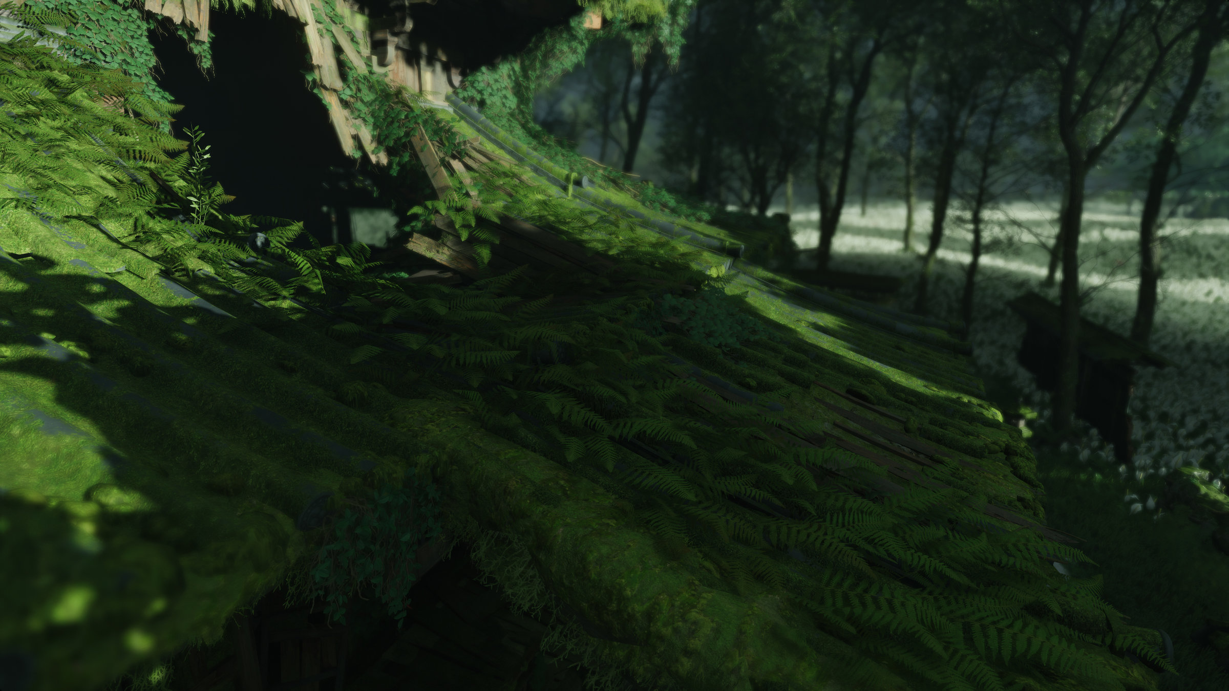
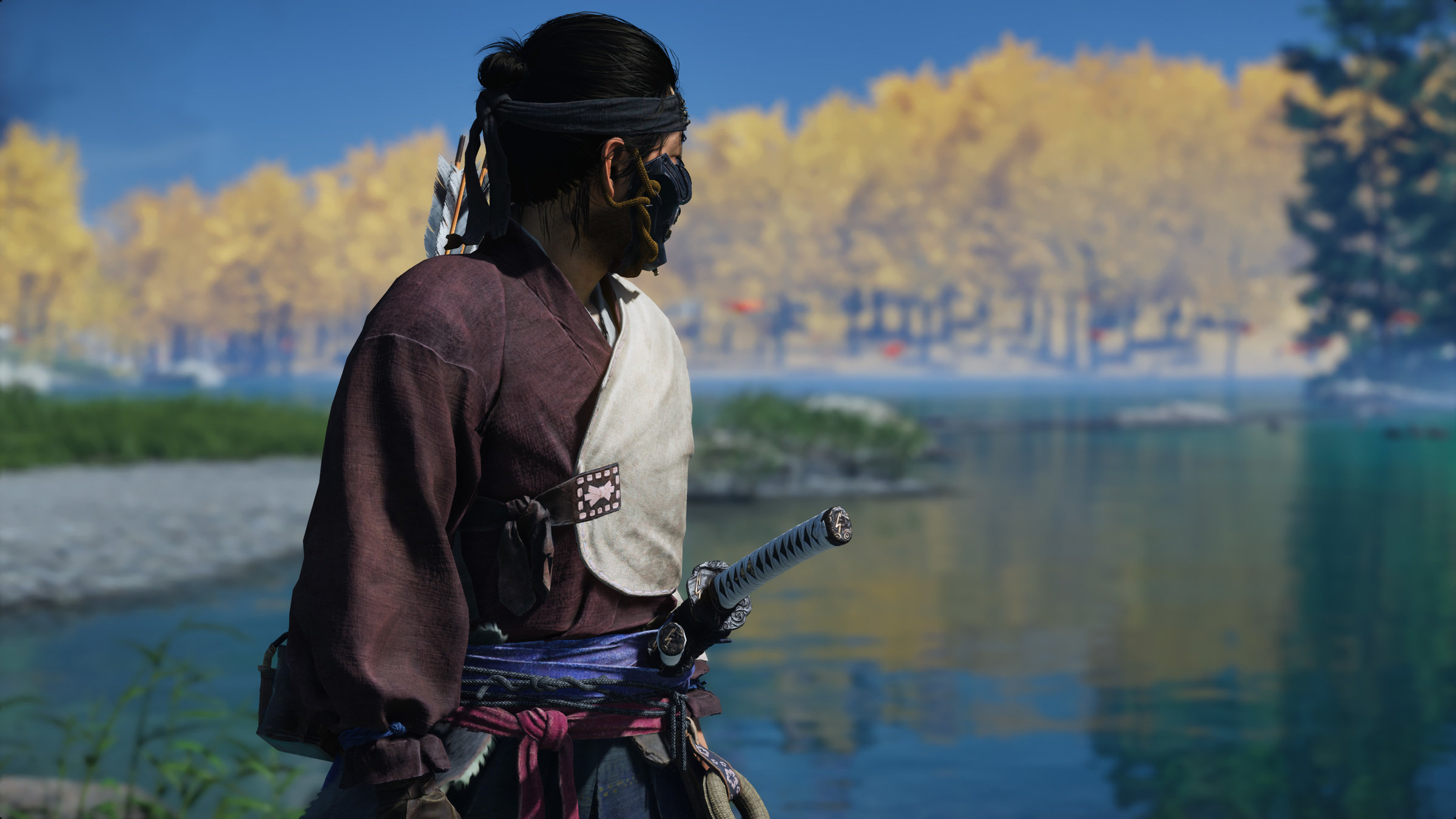
Jasmin Patry
Sucker Punch Productions
in

Samurai Shading
© 2020 Sony Interactive Entertainment LLC. Ghost of Tsushima is a trademark of Sony Interactive Entertainment LLC.

Introduction


Introduction

Introduction | Goals
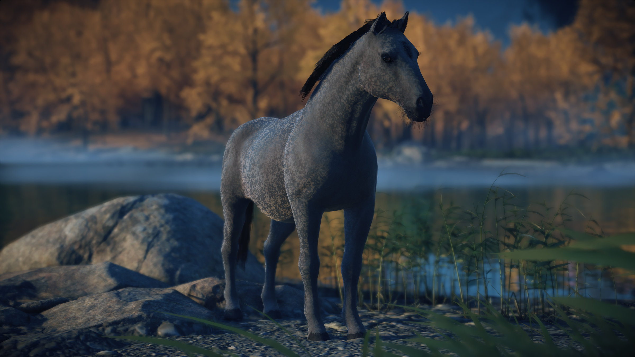
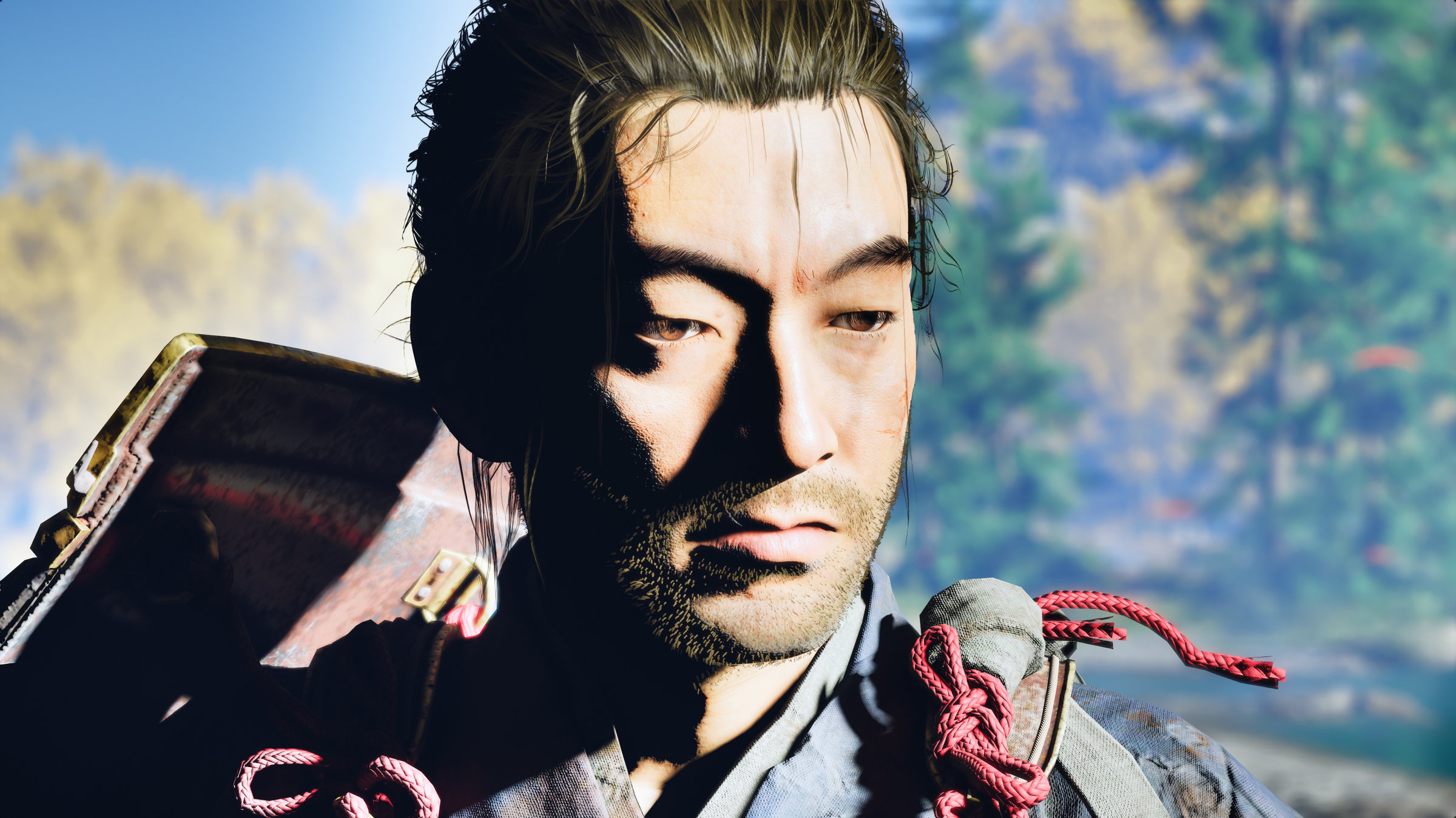
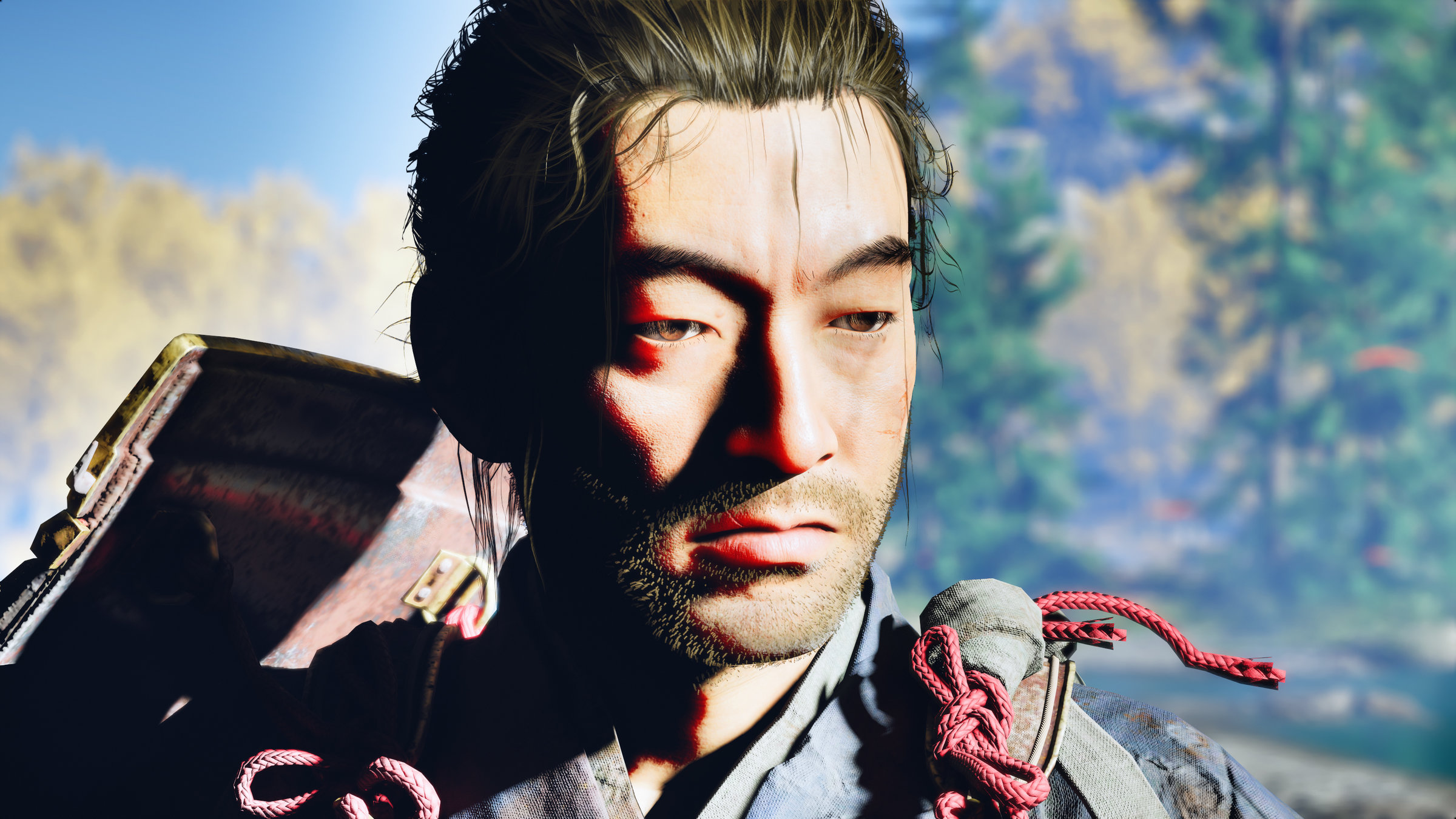
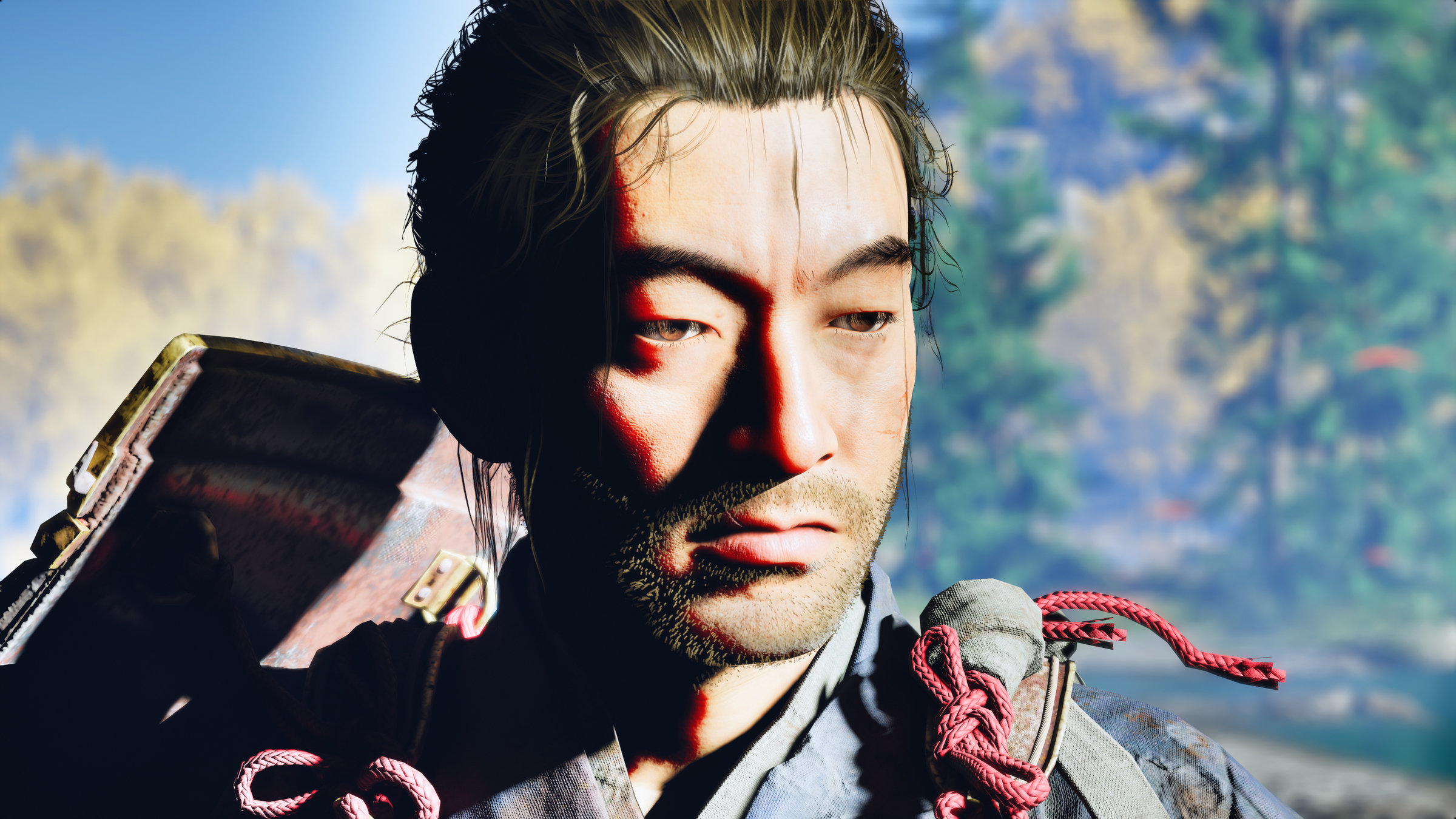
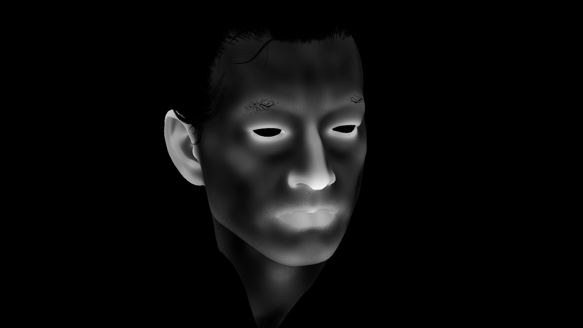
Introduction | Lighting
Introduction | Lighting
Introduction | Overview


Anisotropic Specular
Anisotropic Specular
Anisotropic Specular| Previous Work
Anisotropic Specular| Previous Work
Anisotropic Specular | SGGX Recap
Anisotropic Specular | SGGX Recap
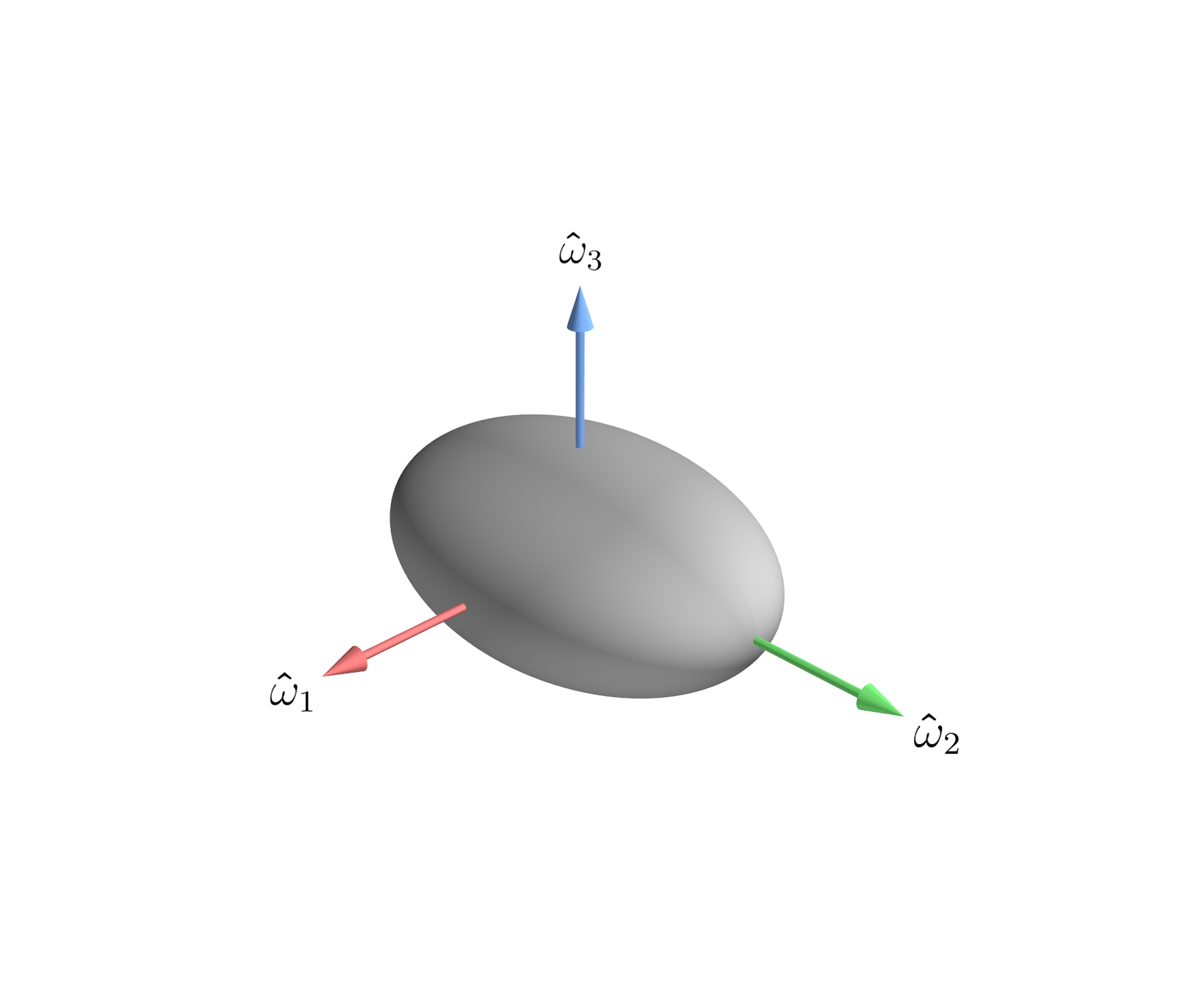
Anisotropic Specular | SGGX Recap
Anisotropic Specular | SGGX Recap
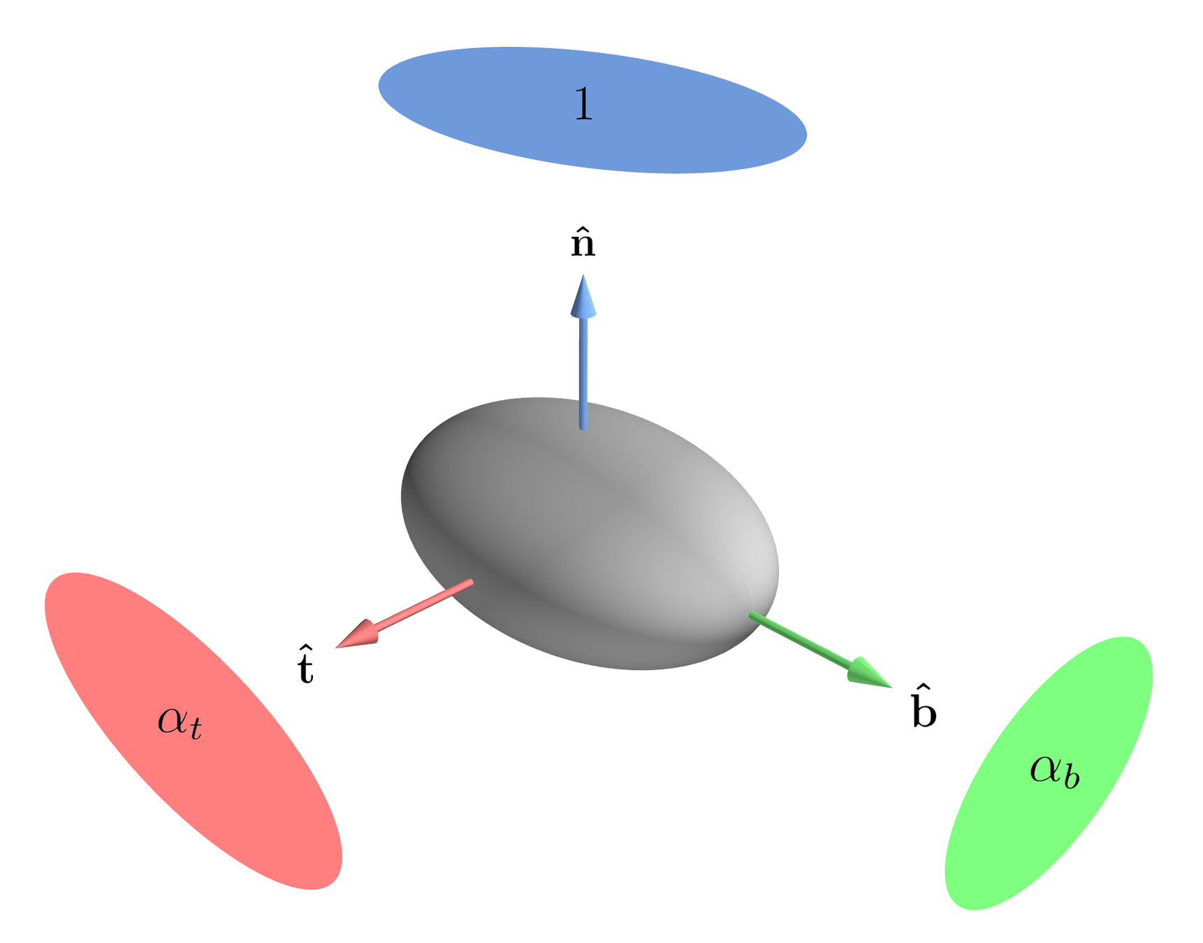
- \(\mathbf{\hat{t}}\): Tangent
- \(\mathbf{\hat{b}}\): Bitangent
- \(\mathbf{\hat{n}}\): Normal
- \(\alpha\): GGX roughness
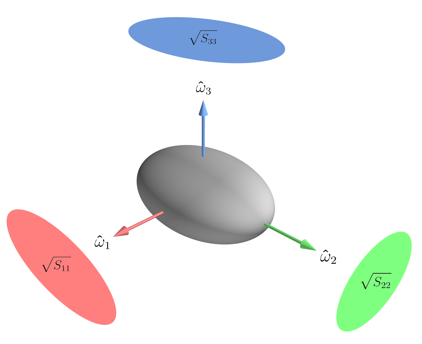
Anisotropic Specular | SGGX Recap
- \(\mathbf{\hat{t}}_n\): Normal-mapped tangent
- \(\mathbf{\hat{b}}_n\): Normal-mapped bitangent
- \(\mathbf{\hat{n}}\): Normal-mapped normal
- \(S_{xx}, S_{xy}, S_{yy}\): 2x2 GGX submatrix
Anisotropic Specular | SGGX Recap
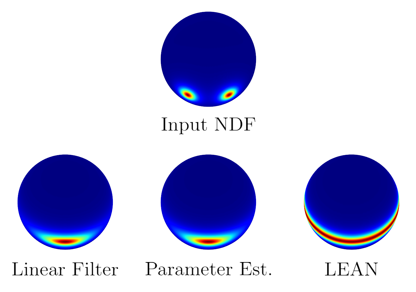
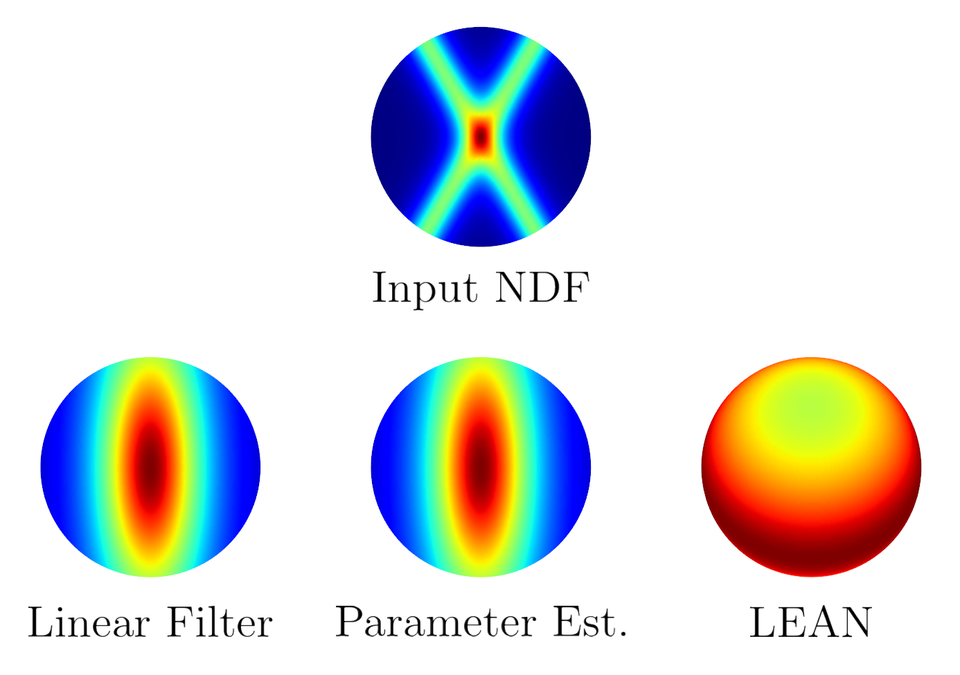
Input NDF
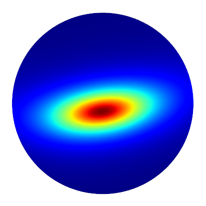
Parameter Estimation
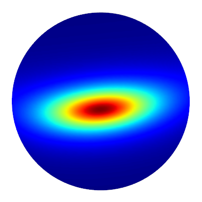
Linear Filtering
Parameter Estimation
Anisotropic Specular| Our Algorithm
Anisotropic Specular| Our Algorithm
Anisotropic Specular| Our Algorithm
Anisotropic Specular| Our Algorithm
Anisotropic Specular| Our Algorithm
void DecodeSggx(float3 anisoTex, float3 tangent, float3 bitangent, out SAnisoSpecData anid)
{
    const float s_alphaMin = GgxAlphaFromGloss(1.0f);

    float sxx = Square(anisoTex.x);
    float sxy = anisoTex.x * (anisoTex.y * 2.0 - 1.0) * anisoTex.z;
    float syy = Square(anisoTex.z);

    float discr = sqrt(4.0f * Square(sxy) + Square(sxx - syy));
    float discrRcp = rcp(max(discr, 1e-6f));

    anid.m_alphaTSqr = max(saturate(0.5f * (sxx + syy + discr)), Square(s_alphaMin));
    anid.m_alphaBSqr = max(saturate(0.5f * (sxx + syy - discr)), Square(s_alphaMin));
    anid.m_alphaTB = sqrt(anid.m_alphaTSqr * anid.m_alphaBSqr);

    float cSqr = saturate(0.5f * ((sxx - syy) * discrRcp + 1.0f));
    float c = sqrt(cSqr);
    float s = Sign(sxy) * sqrt(1.0f - cSqr);

    anid.m_tangent = c * tangent + s * bitangent;
    anid.m_bitangent = -s * tangent + c * bitangent;
}
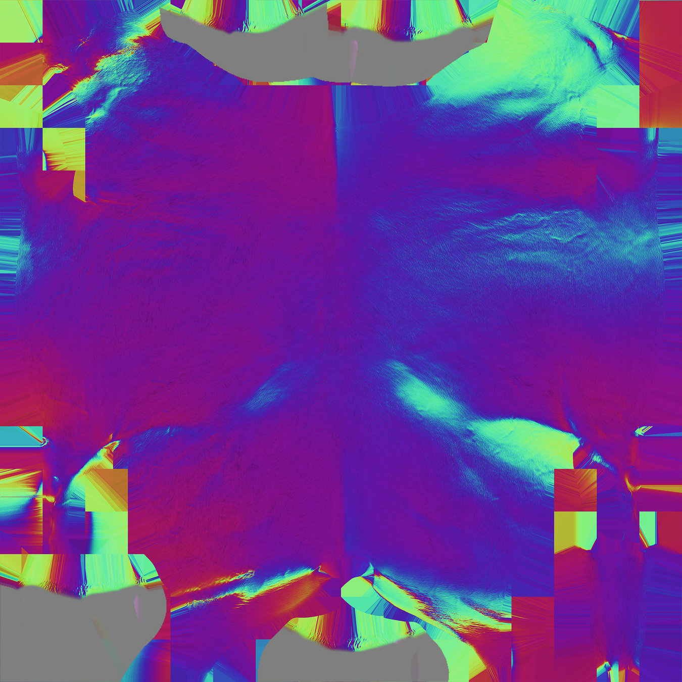
Anisotropic Specular| Authoring
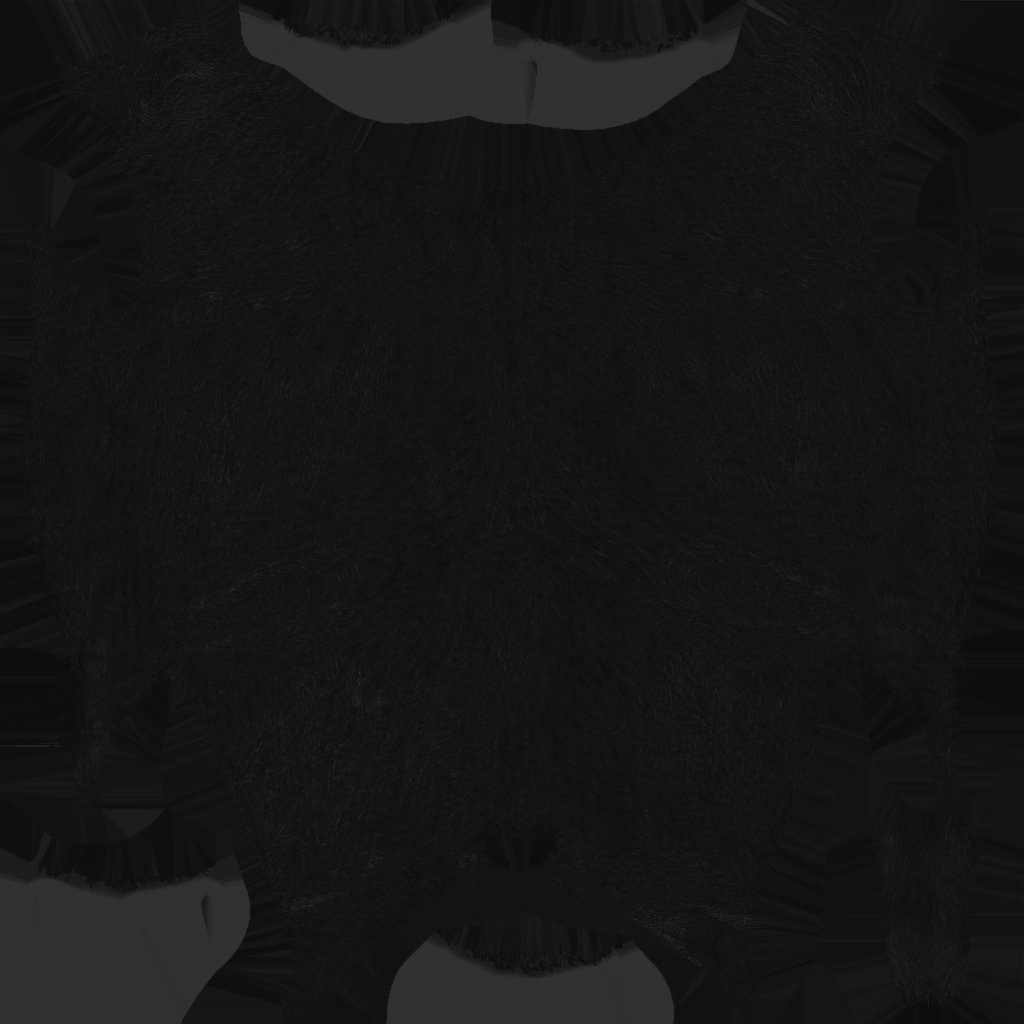
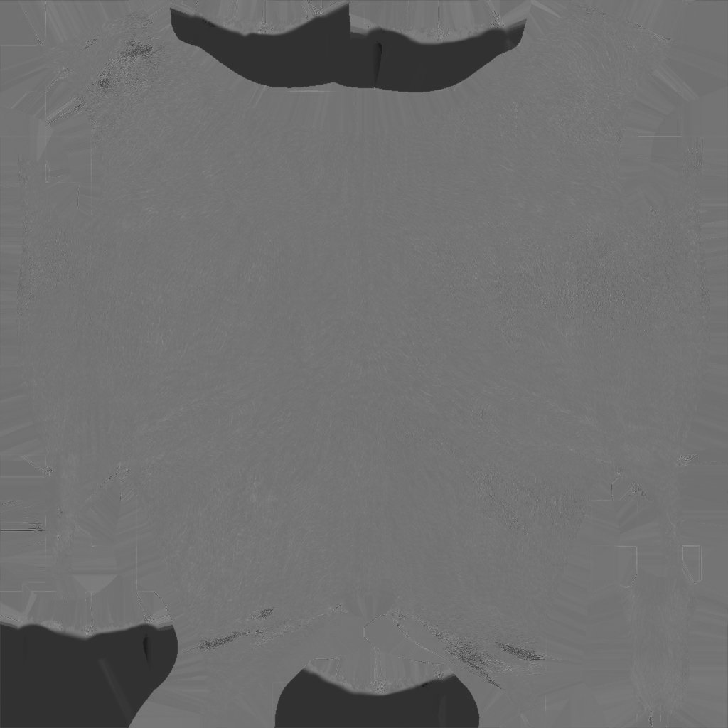
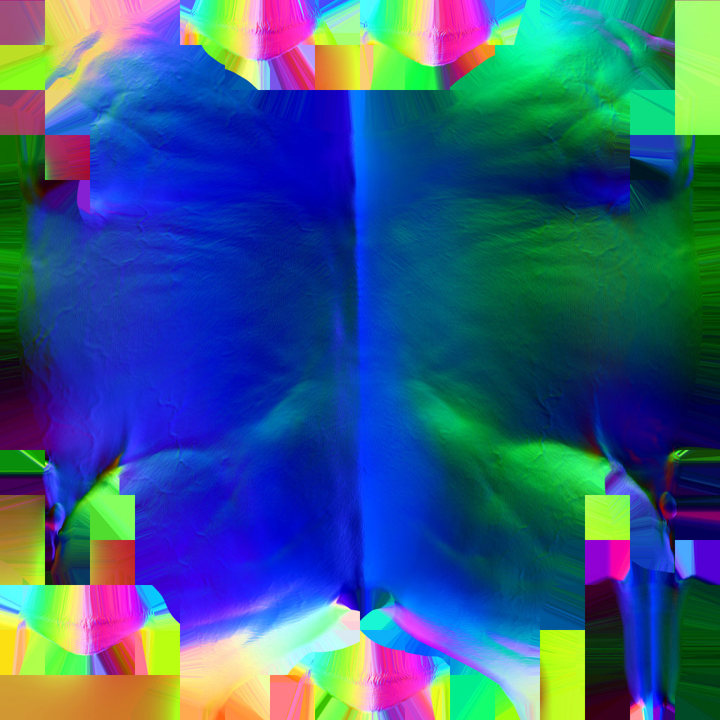
Gloss U
Gloss V
Direction
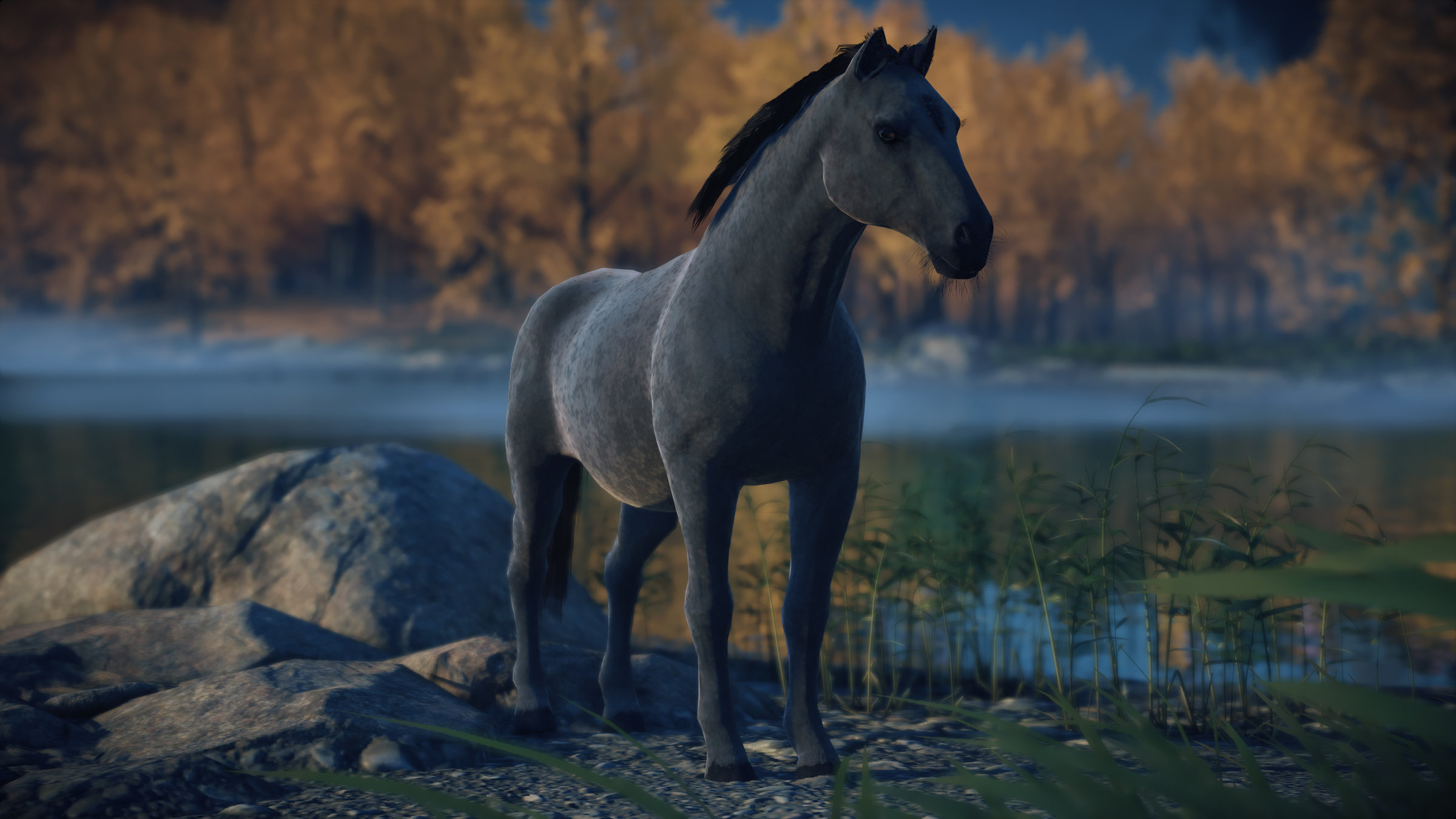
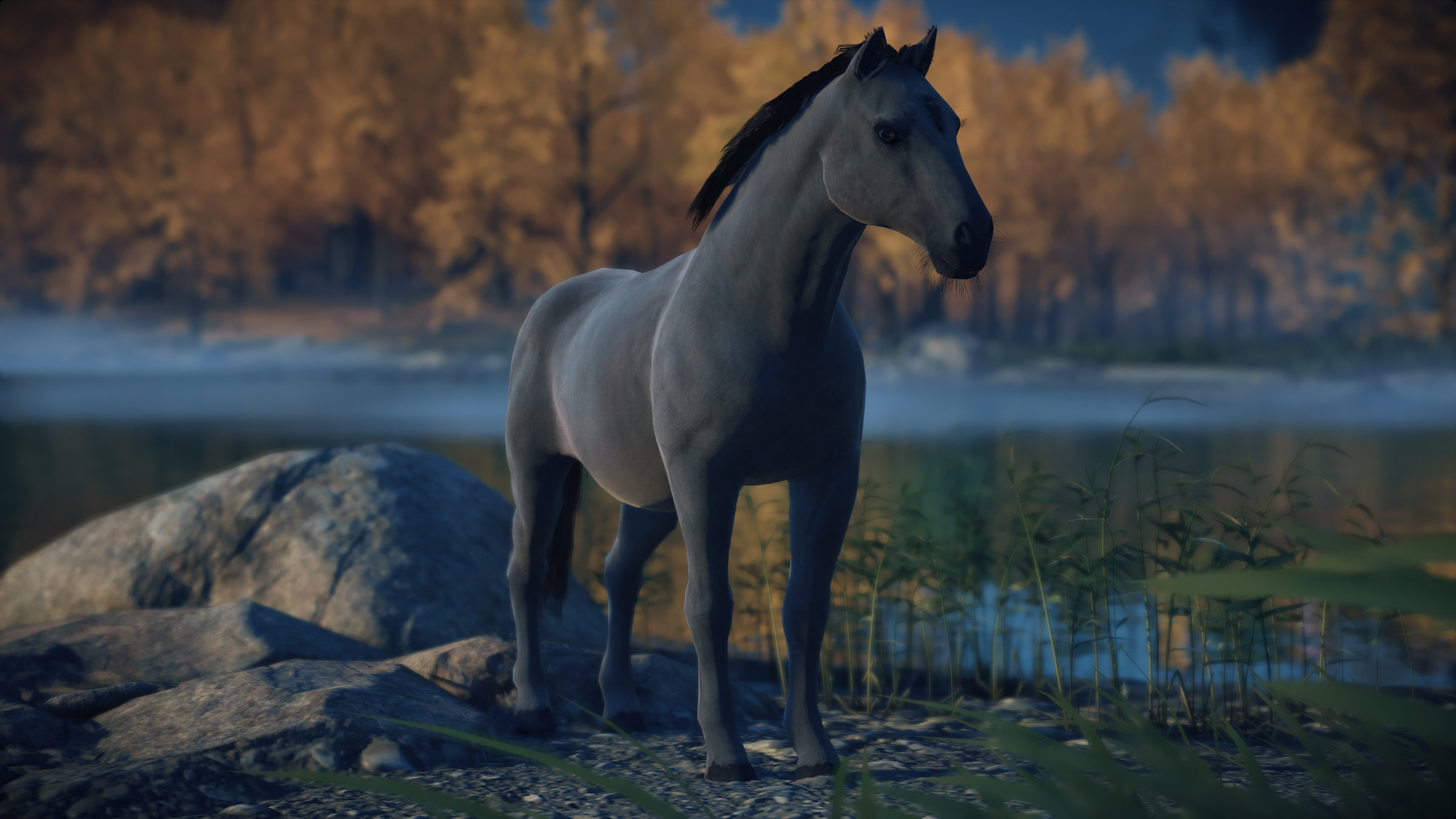
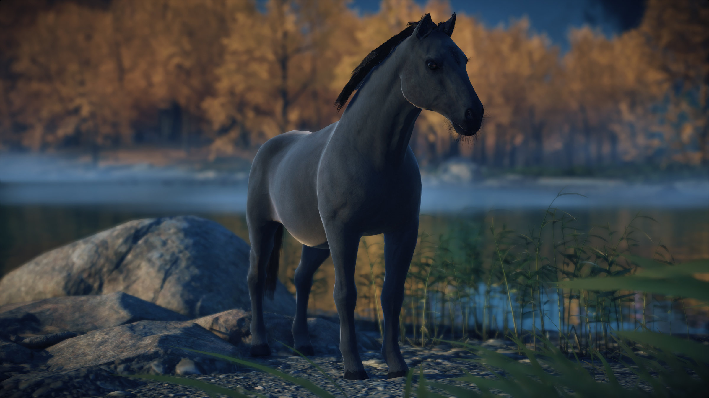
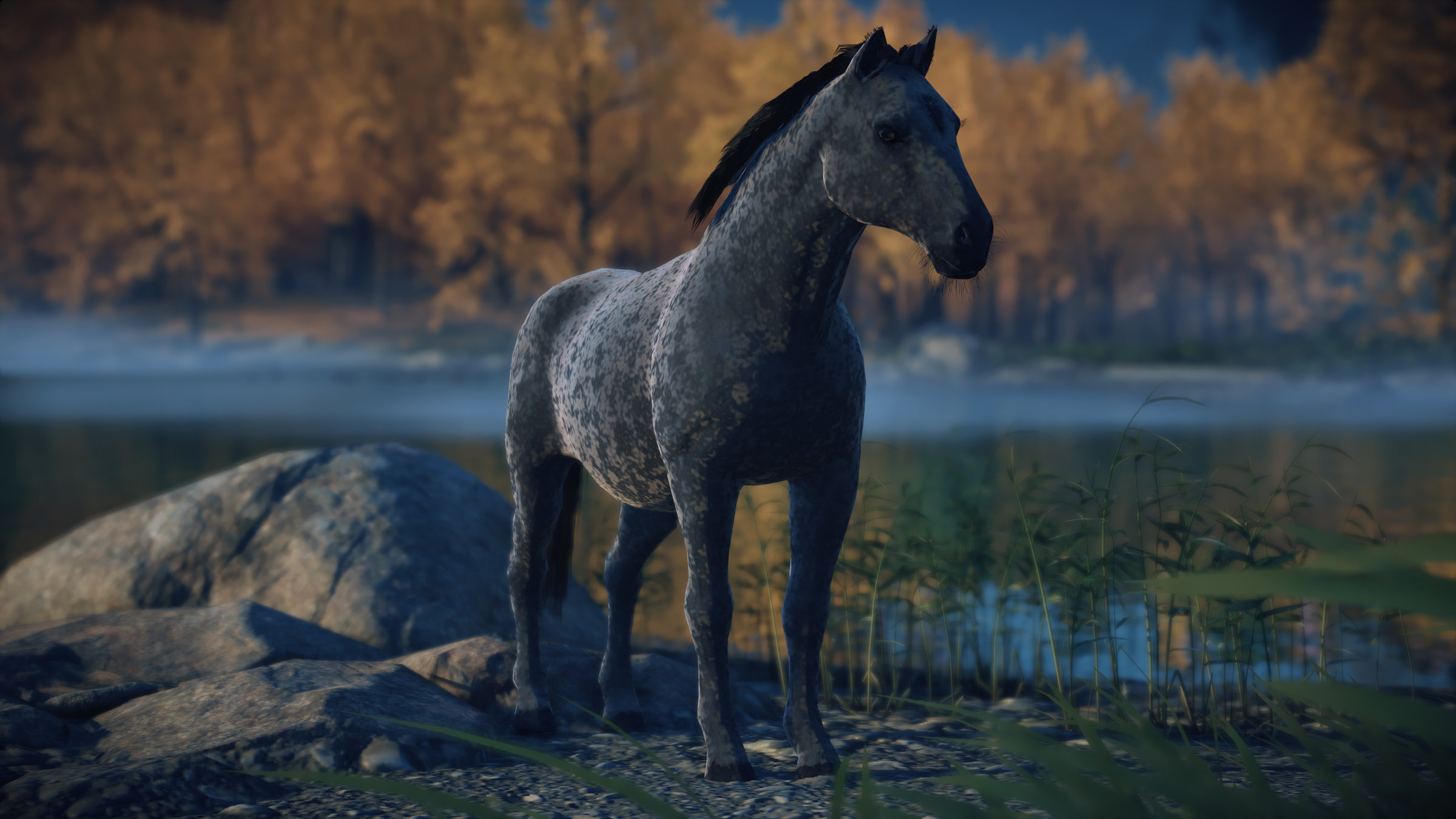
Aniso
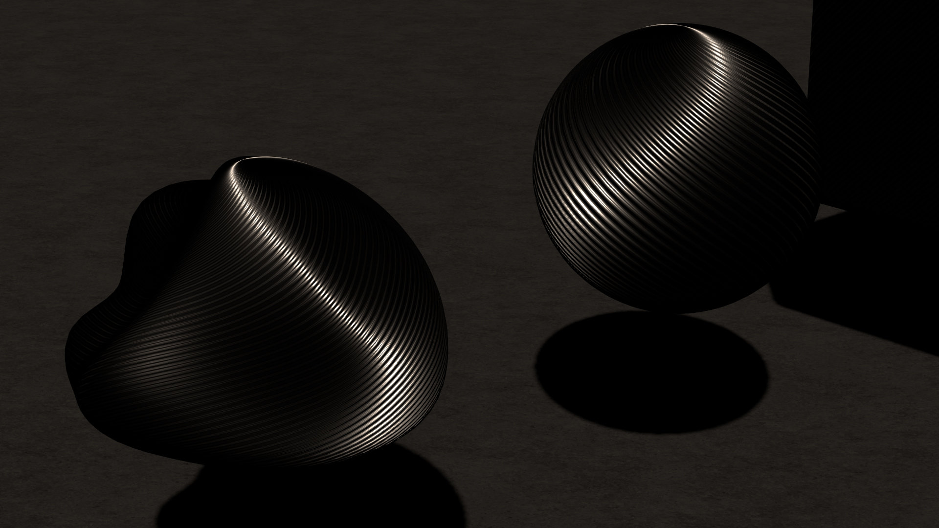
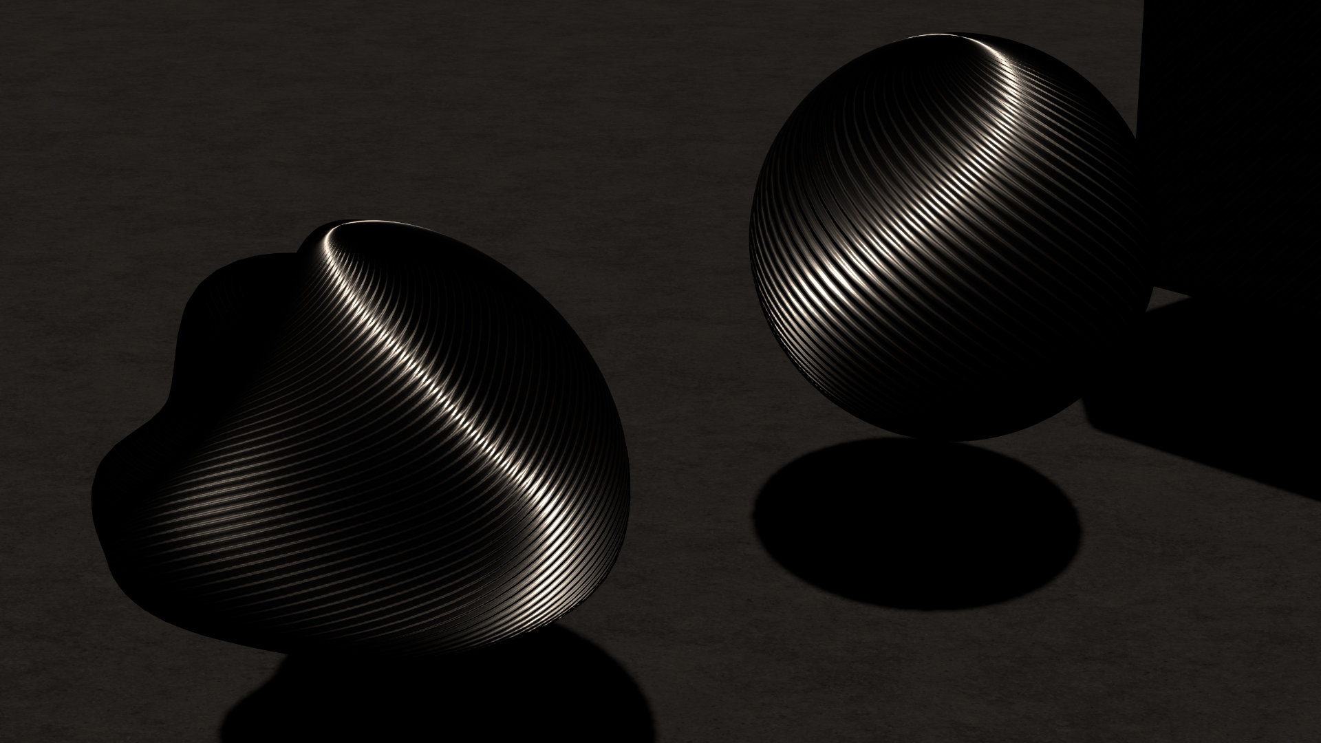
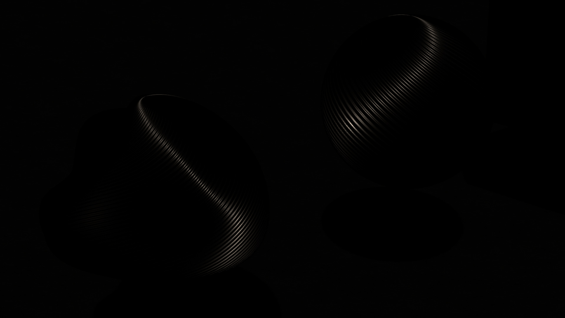
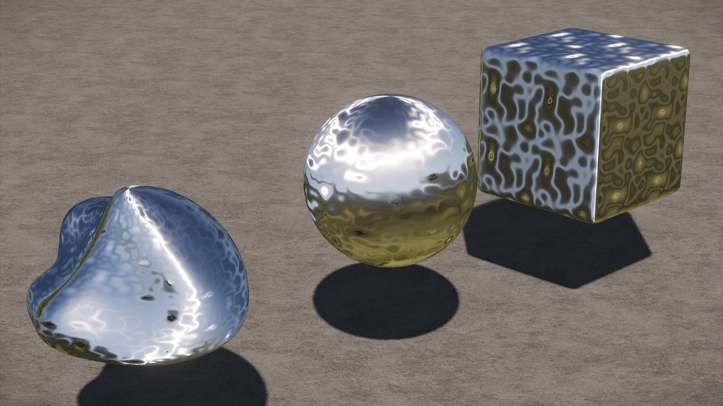
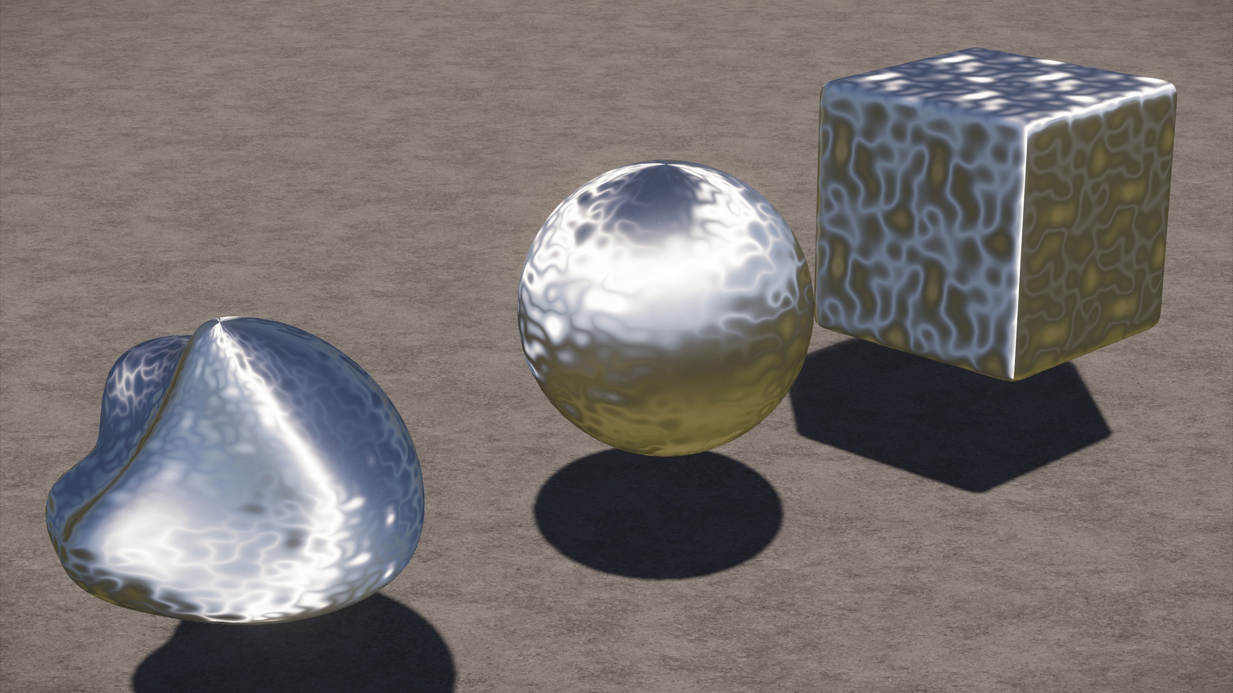
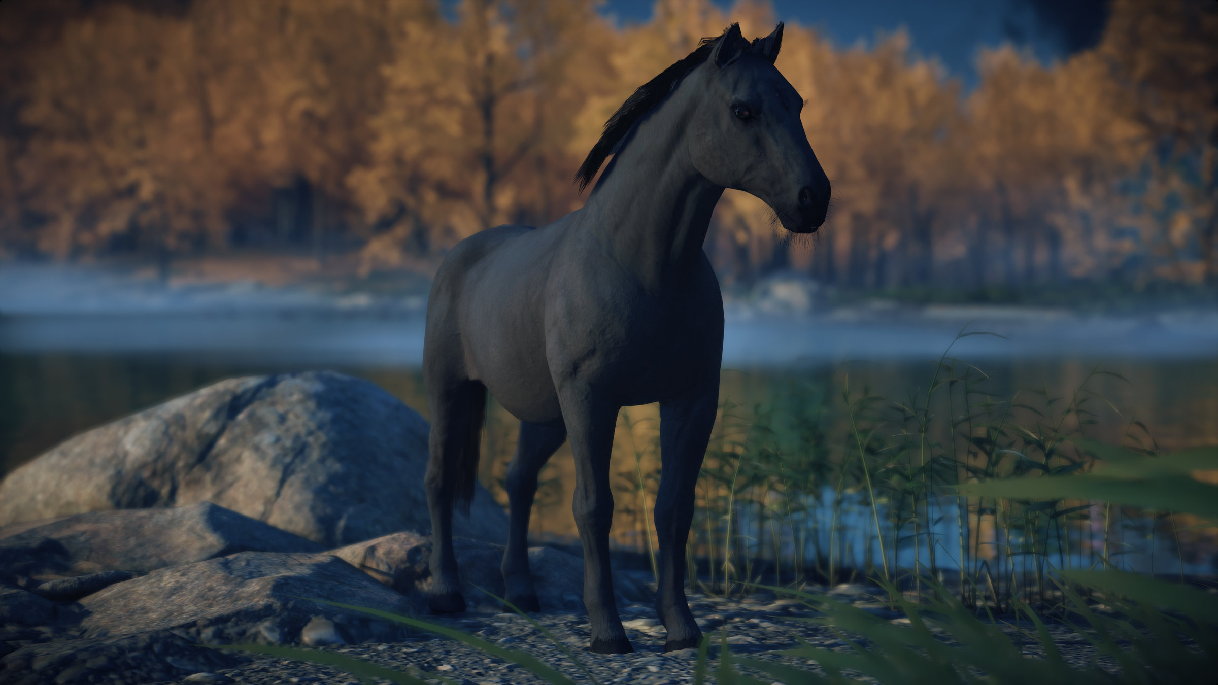
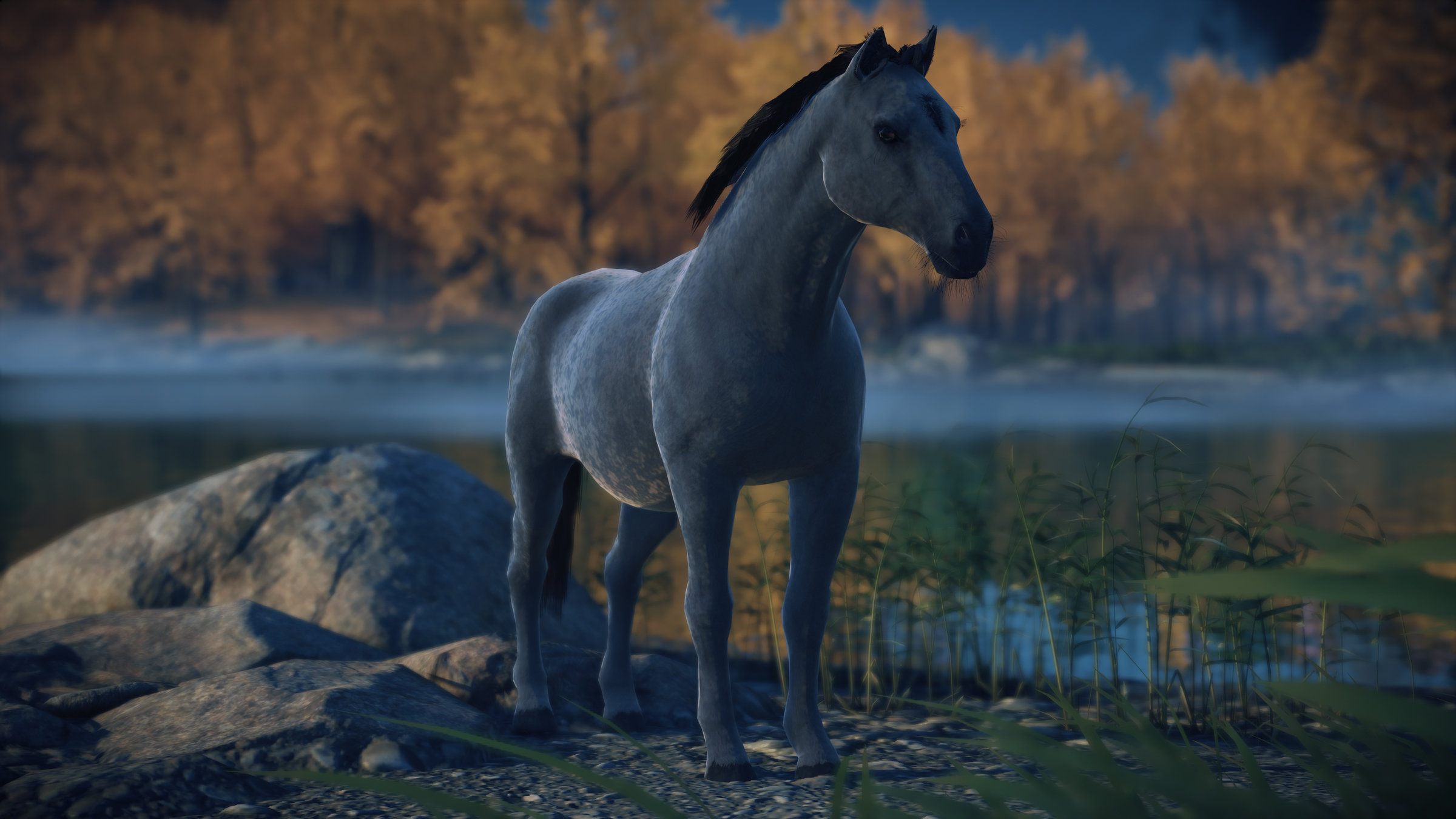
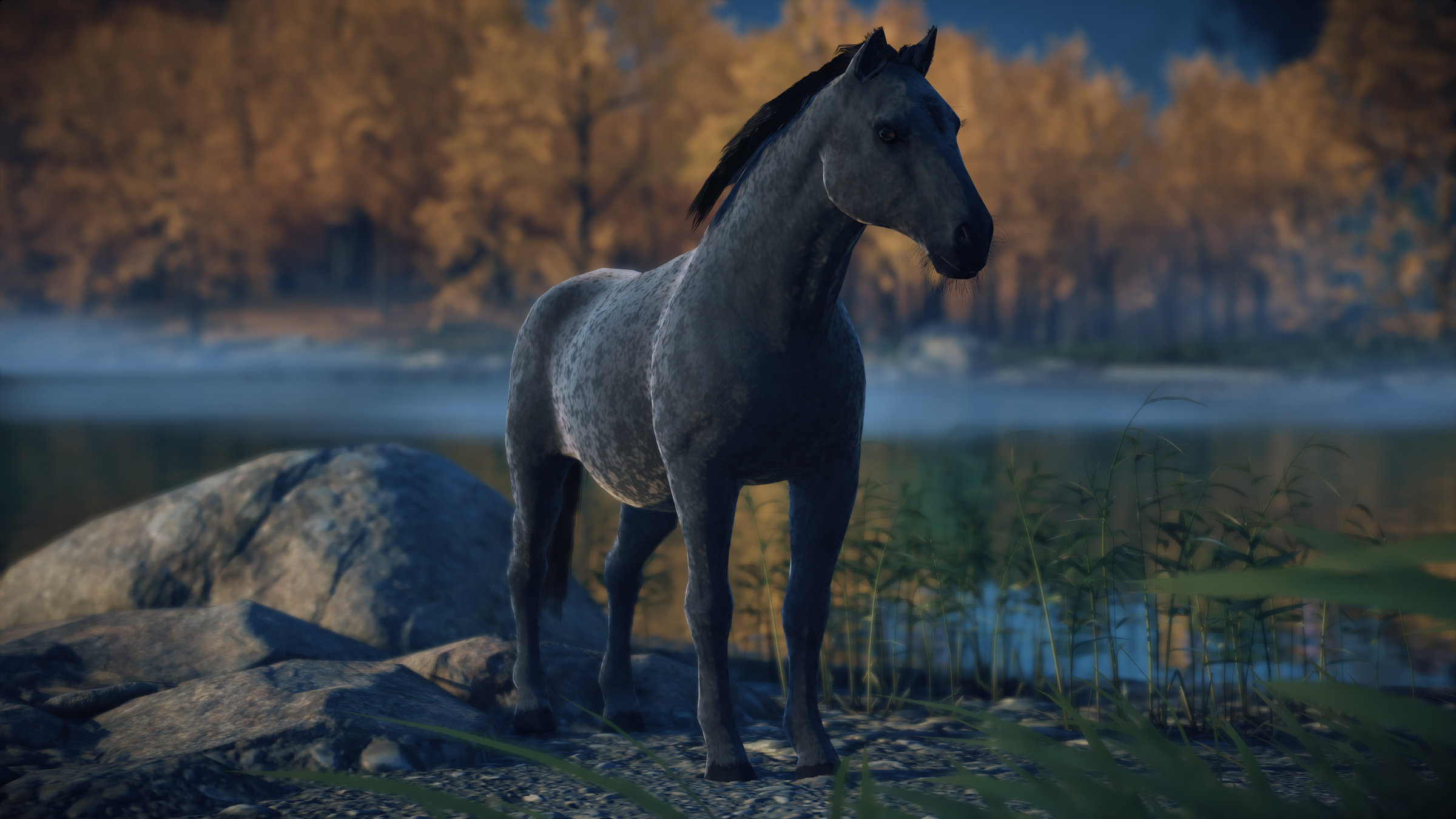
Anisotropic Specular| Results
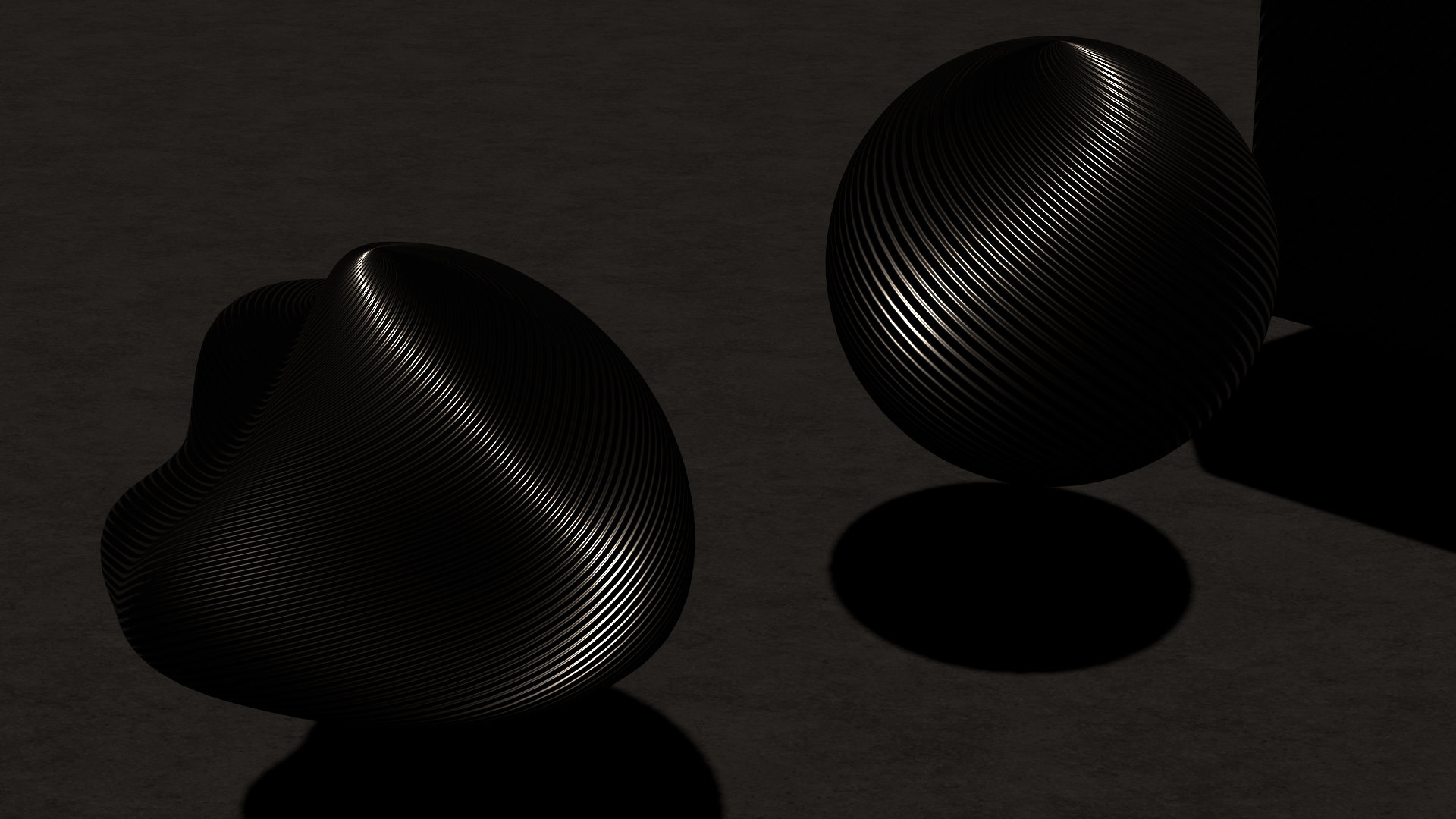
Ground Truth (256 samples per pixel)
SGGX (ours)
LEAN
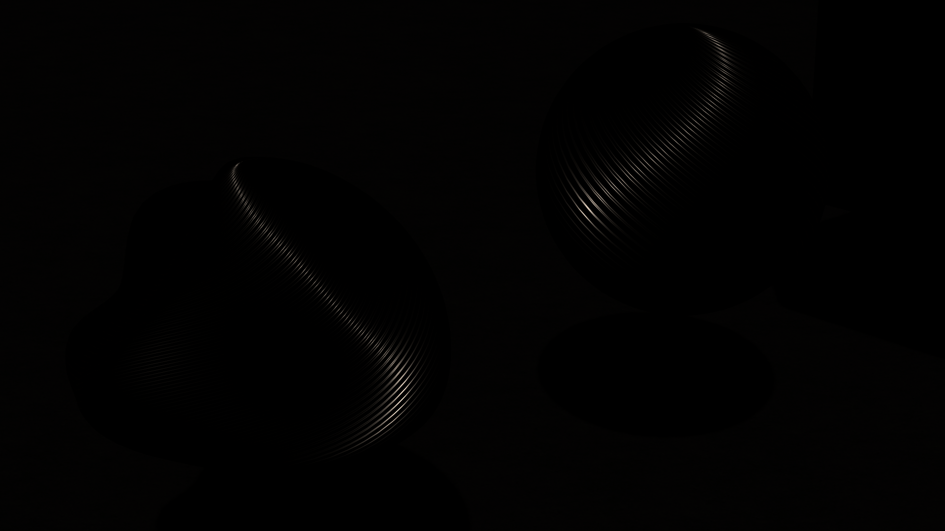
Ground Truth (256 samples per pixel)
SGGX (ours)
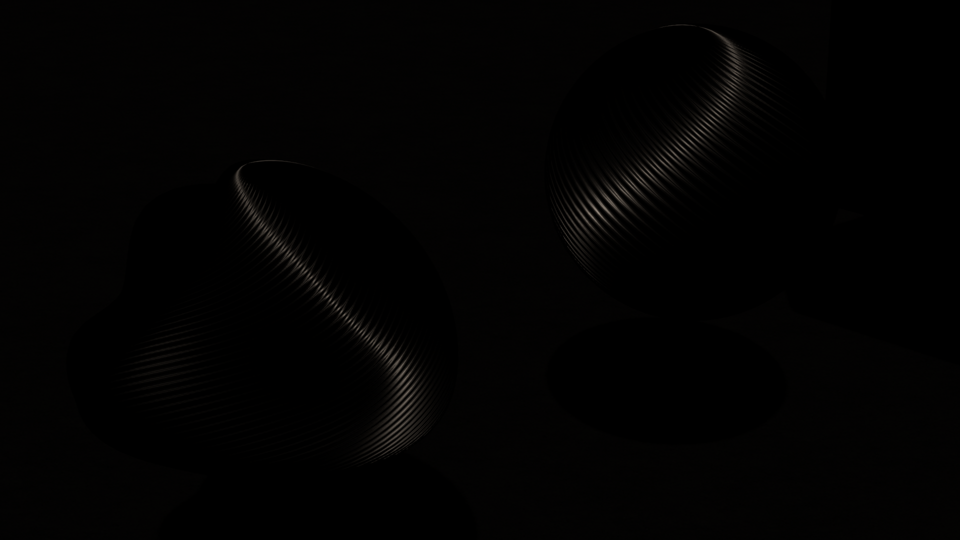
LEAN
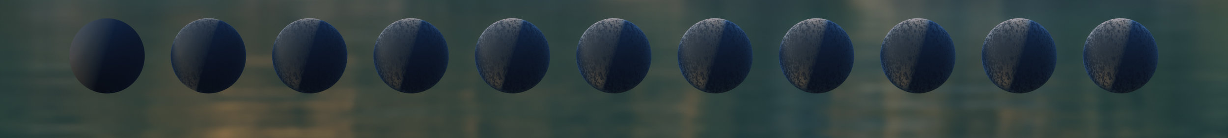
Anisotropic Specular| Limitations

\(\alpha_t = 0.29, \alpha_b = 0.04\)
\(\alpha_t = 0.87, \alpha_b = 0.04\)
\(\alpha_t = 0.87, \alpha_b = 0.1\)
Anisotropic Specular| Summary
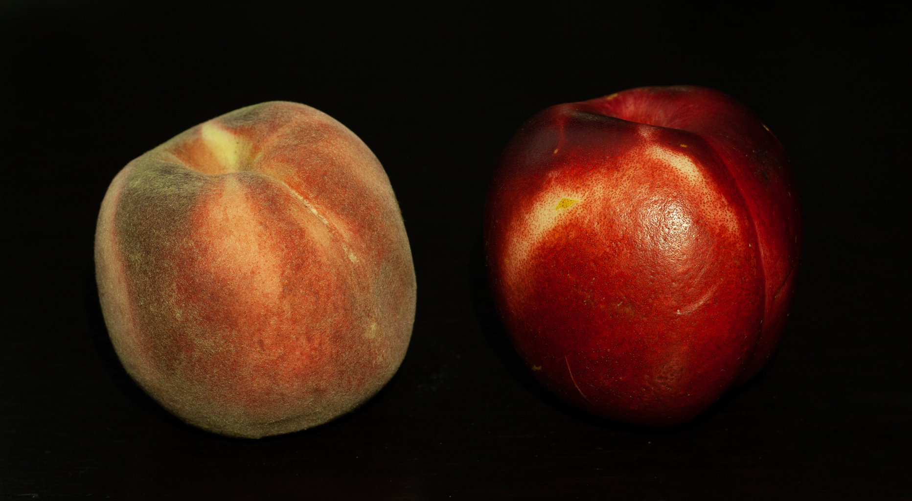
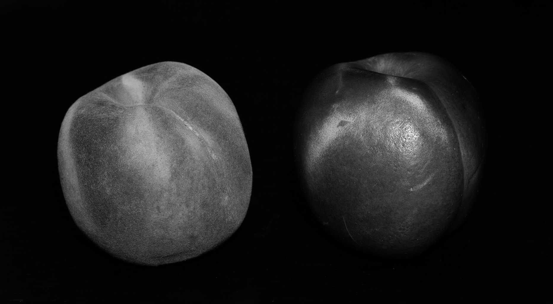
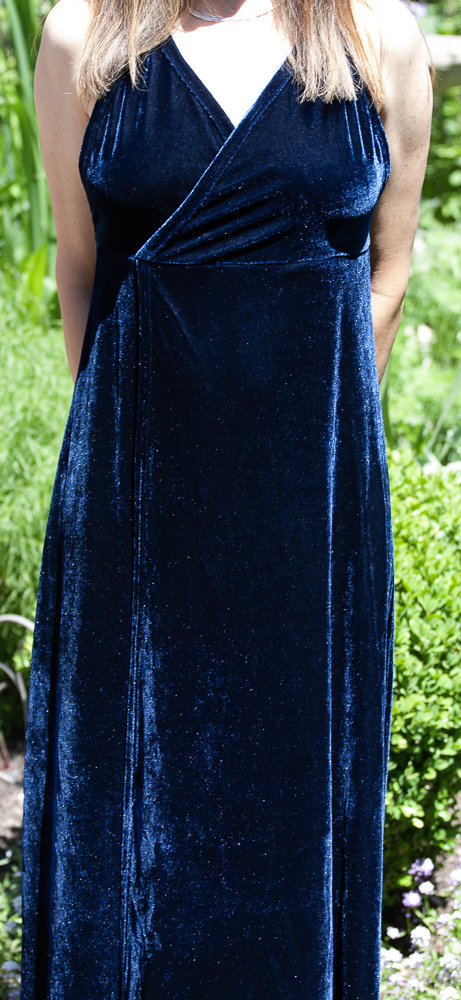
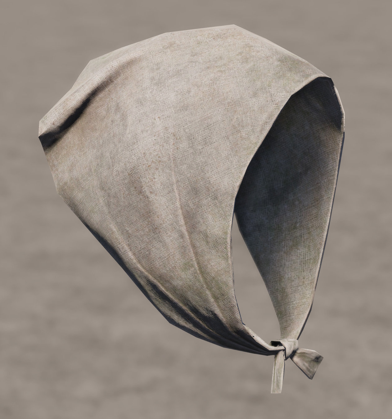
Anisotropic Asperity Scattering
Anisotropic
Asperity Scattering BRDF
Anisotropic
Asperity Scattering BRDF
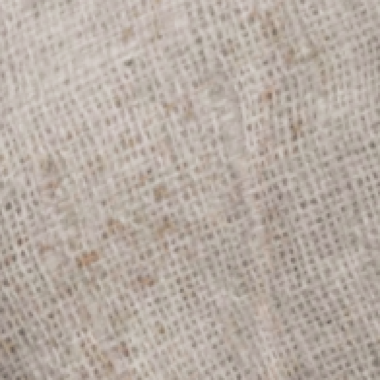
Fuzz
Anisotropic
Asperity Scattering BRDF
Fuzz
Anisotropic
Asperity Scattering BRDF
Fuzz
Anisotropic
Asperity Scattering BRDF
Fuzz
Anisotropic Fuzz | Previous Work
Anisotropic Fuzz | New Model
- \(\mathbf{\hat{u}}\): Light direction
- \(\mathbf{\hat{v}}\): View direction
- \(p(\mathbf{\hat{u}}, \mathbf{\hat{v}})\): Phase function
- \(\Delta\): Thickness of scattering layer
- \(\lambda\): Mean free path
- \(d = \frac{\Delta}{\lambda} \ll 1\): Density
Base Layer
Scattering Layer
Anisotropic Fuzz | New Model
Base Layer
Scattering Layer
- \(\mathbf{\hat{u}}\): Light direction
- \(\mathbf{\hat{v}}\): View direction
- \(p(\mathbf{\hat{u}}, \mathbf{\hat{v}})\): Phase function
- \(\Delta\): Thickness of scattering layer
- \(\lambda\): Mean free path
- \(d = \frac{\Delta}{\lambda} \ll 1\): Density
- \(\mathbf{c}_f\): Albedo

Anisotropic Fuzz | New Model
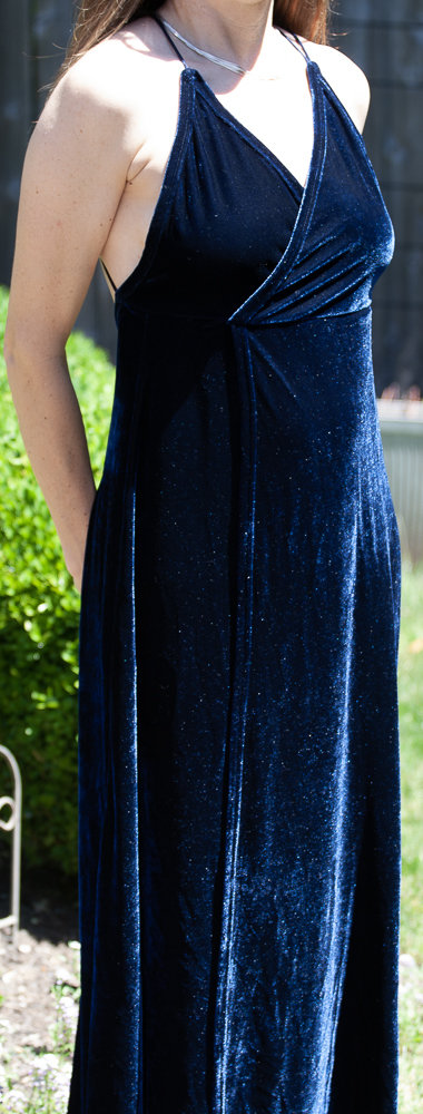
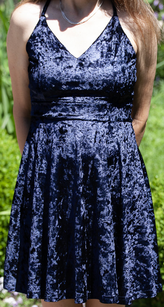
Anisotropic Fuzz | Velvet Scattering

Anisotropic Fuzz | Velvet Scattering
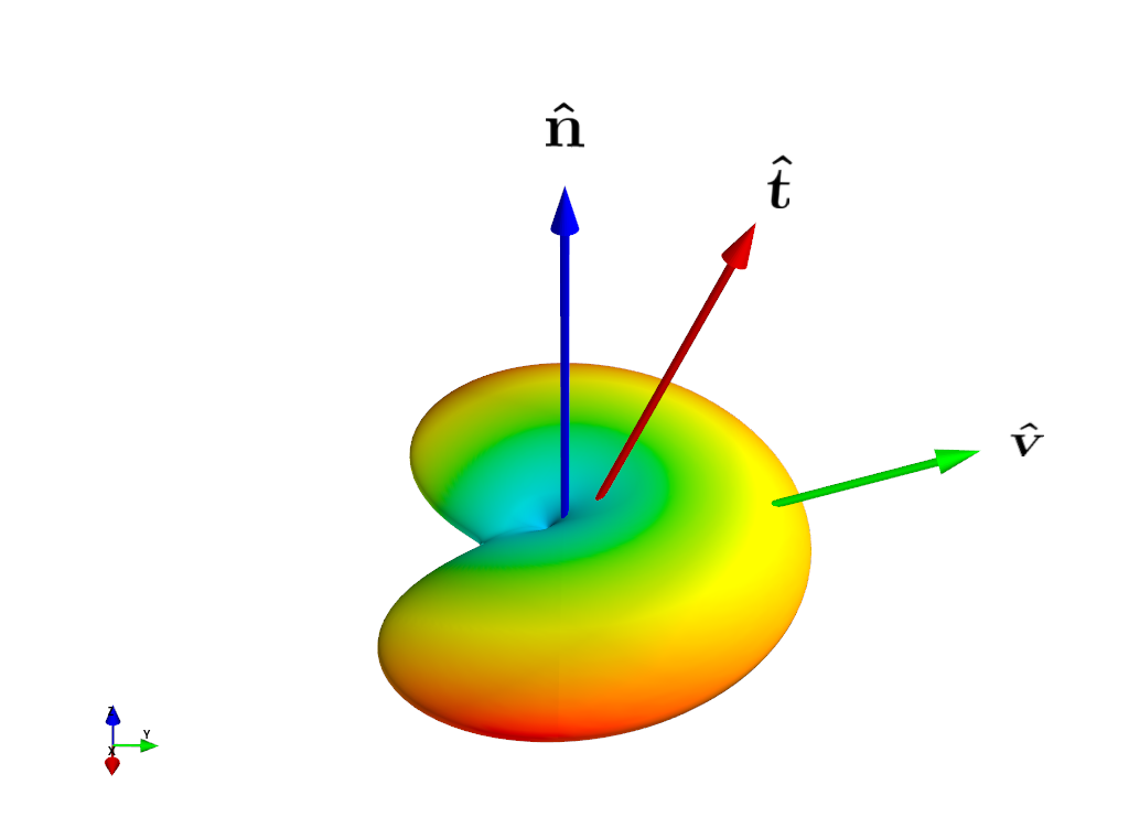
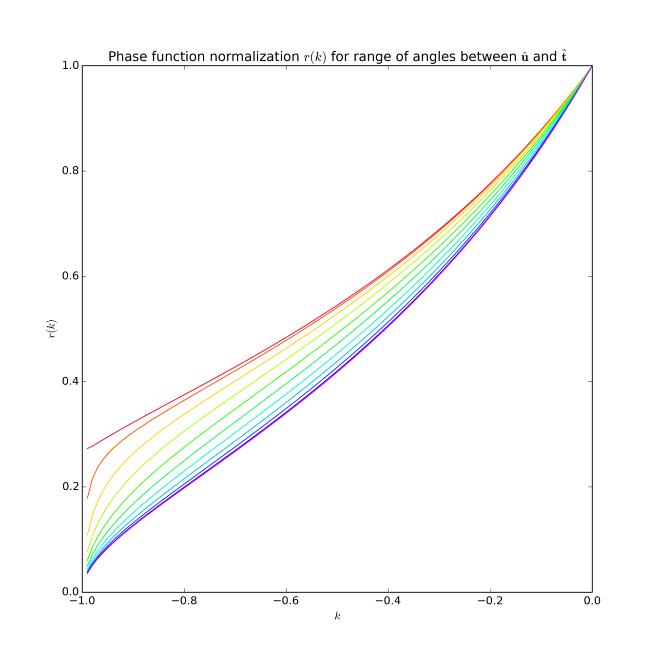
Anisotropic Fuzz | Phase Function
Anisotropic Fuzz | Phase Function

Anisotropic Fuzz | Phase Function
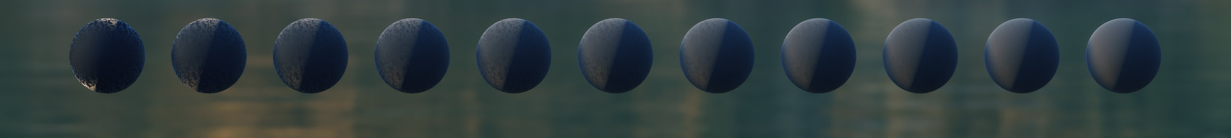
Vary Schlick \(k\)
Vary Fiber (\(\mathbf{\hat{t}}\)) Polar Angle
Vary View (\(\mathbf{\hat{v}}\)) Polar Angle
Vary View (\(\mathbf{\hat{v}}\)) Azimuthal Angle
Anisotropic Fuzz | Phase Function
Anisotropic Fuzz | Phase Function
- \(\mathbf{\hat{u}}\): Light direction
- \(\mathbf{\hat{v}}\): View direction
- \(\mathbf{\hat{h}}=\frac{\mathbf{\hat{u}}+\mathbf{\hat{v}}}{\left|\mathbf{\hat{u}}+\mathbf{\hat{v}}\right|}\): Half vector
- \(\mathbf{\hat{t}}\): Fiber direction
- \(\alpha\): GGX roughness
- \(D_F\): (S)GGX “fiber” NDF
- \(\sigma_F\): Microflake projected area
- \(p_F(\mathbf{\hat{u}}, \mathbf{\hat{v}})\): Phase function
Anisotropic Fuzz | Phase Function

Anisotropic Fuzz | Phase Function
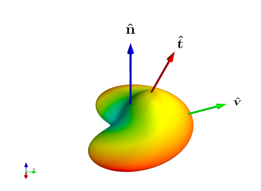
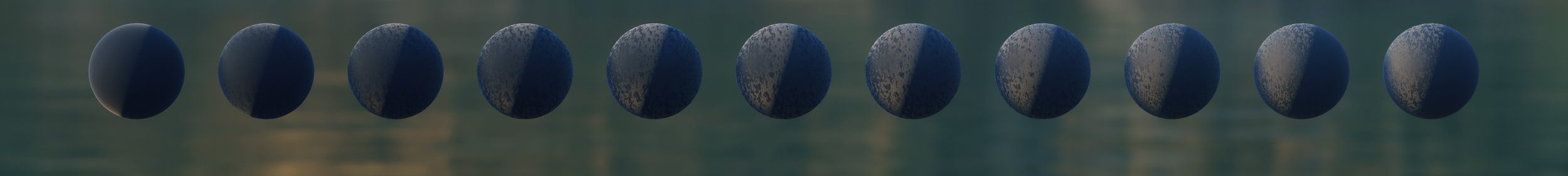
Vary \(\alpha\)
Vary Fiber (\(\mathbf{\hat{t}}\)) Polar Angle
Vary View (\(\mathbf{\hat{v}}\)) Polar Angle
Vary View (\(\mathbf{\hat{v}}\)) Azimuthal Angle
Anisotropic Fuzz | Shadowing
Anisotropic Fuzz | Shadowing
Anisotropic Fuzz | Ambient Lighting
Anisotropic Fuzz | Ambient Lighting
Anisotropic Fuzz | Ambient Lighting
Anisotropic Fuzz | Ambient Lighting
Anisotropic Fuzz | Ambient Shadowing
Anisotropic Fuzz | Ambient Shadowing
Bonus Slide
Anisotropic Fuzz | Ambient Shadowing
Bonus Slide
Anisotropic Fuzz | Ambient Shadowing
Bonus Slide
Anisotropic Fuzz | Ambient Shadowing
Bonus Slide
Anisotropic Fuzz | Ambient Shadowing
Bonus Slide
Anisotropic Fuzz | Ambient Shadowing
Bonus Slide
Anisotropic Fuzz | Ambient Shadowing
Bonus Slide
Anisotropic Fuzz | Simplified Deferred Version
Anisotropic Fuzz | Simplified Deferred Version
Anisotropic Fuzz | Simplified Deferred Version
Anisotropic Fuzz | Results
No Fuzz

Fuzziness Enabled With Parameters:
- Density: 0.2
- Spread: 0.2
- Fiber Tilt: 23 degrees
- Noisy Fiber Direction Map
No Base Layer Attenuation
Enabled Base Layer Attenuation
\(P_s(\mathbf{\hat{u}}) \equiv 0\)
\(P_s(\mathbf{\hat{u}})\) implemented
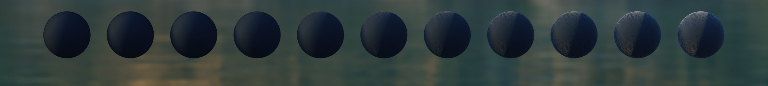
Vary Density \(d \;[0.0, 0.5]\)
Vary Spread \([0.0, 1.0]\)
Vary Fiber Tilt \(\theta_t \;[0.0, 90.0\degree]\)
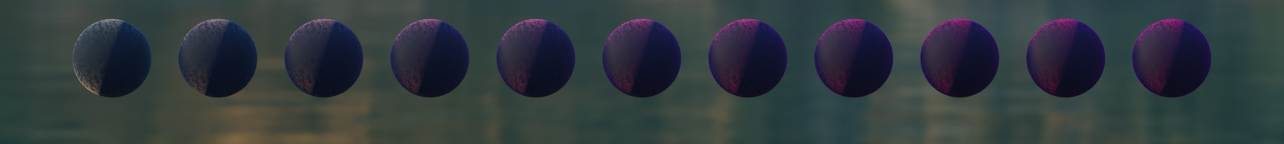
Vary Fiber Color Saturation
Vary Fiber Color Value

Density: 0.1
Density: 0.2
Spread: 0.5
Spread: 1.0
Spread: 0.2
Fiber Tilt: 0 degrees
Fiber Tilt: 45 degrees
Fiber Tilt: 90 degrees
Fiber Tilt: 23 degrees
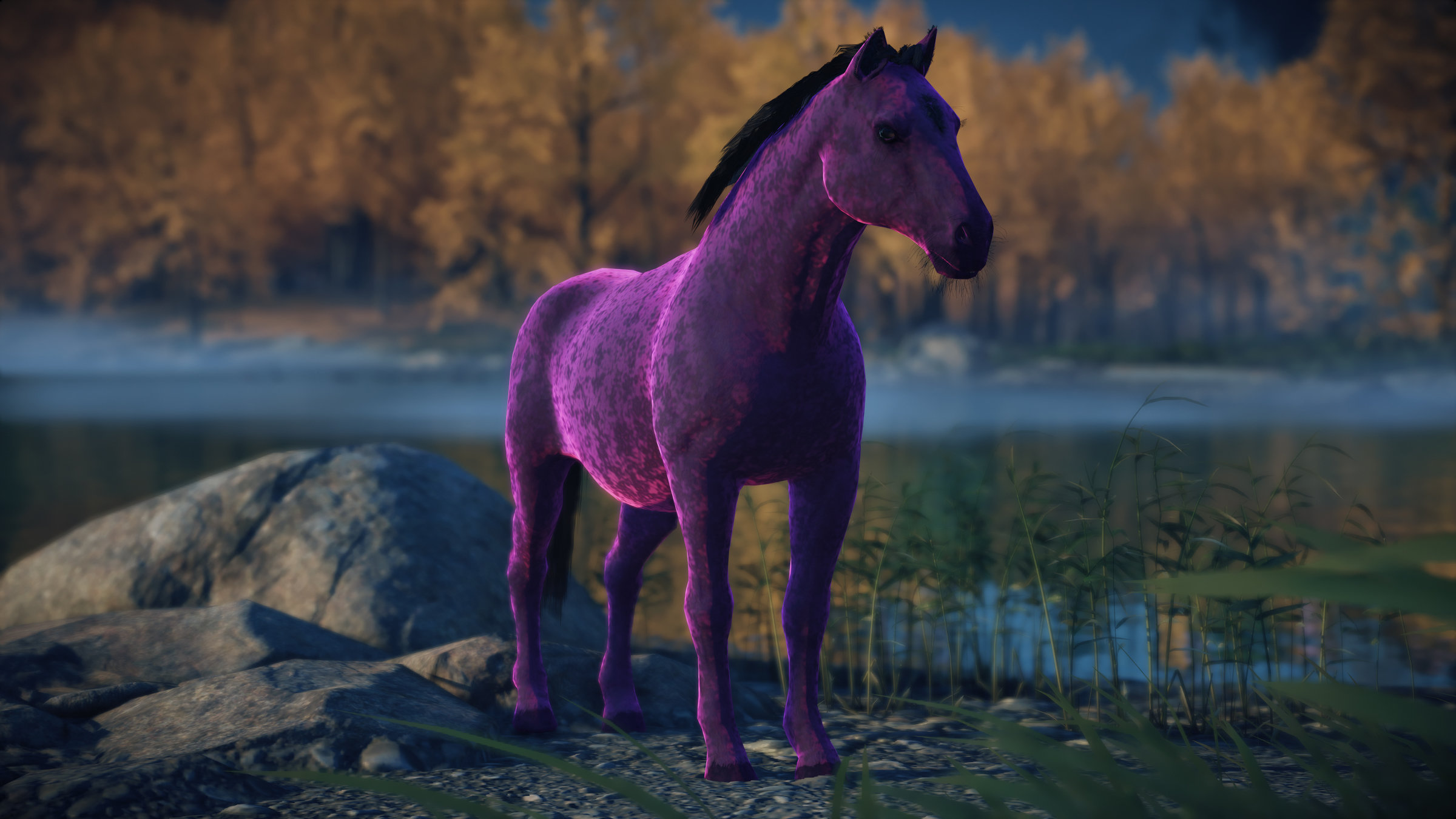
Fiber Color: Hot Pink
Deferred Fuzziness On
Deferred Fuzziness Off
Deferred Fuzziness On
Deferred Fuzziness Off
Anisotropic Fuzz | Summary
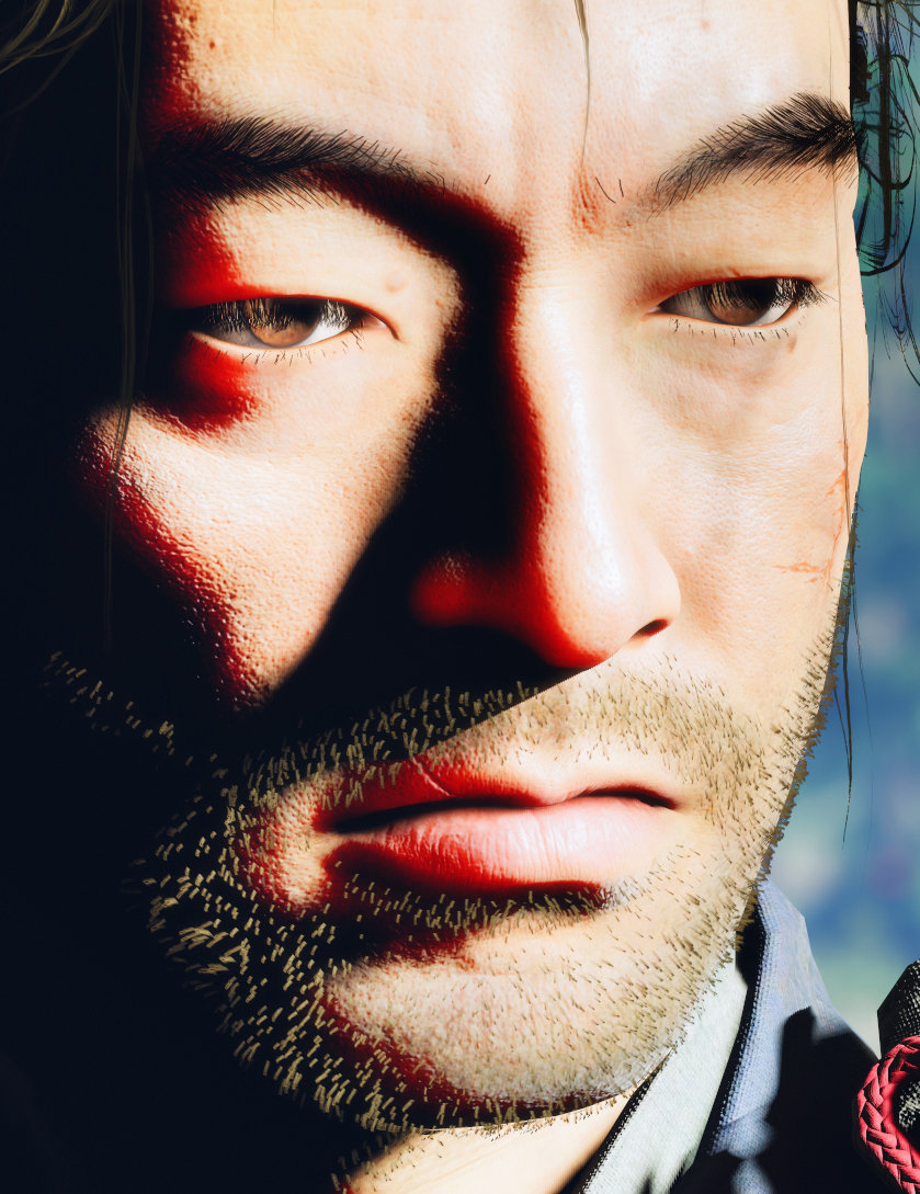
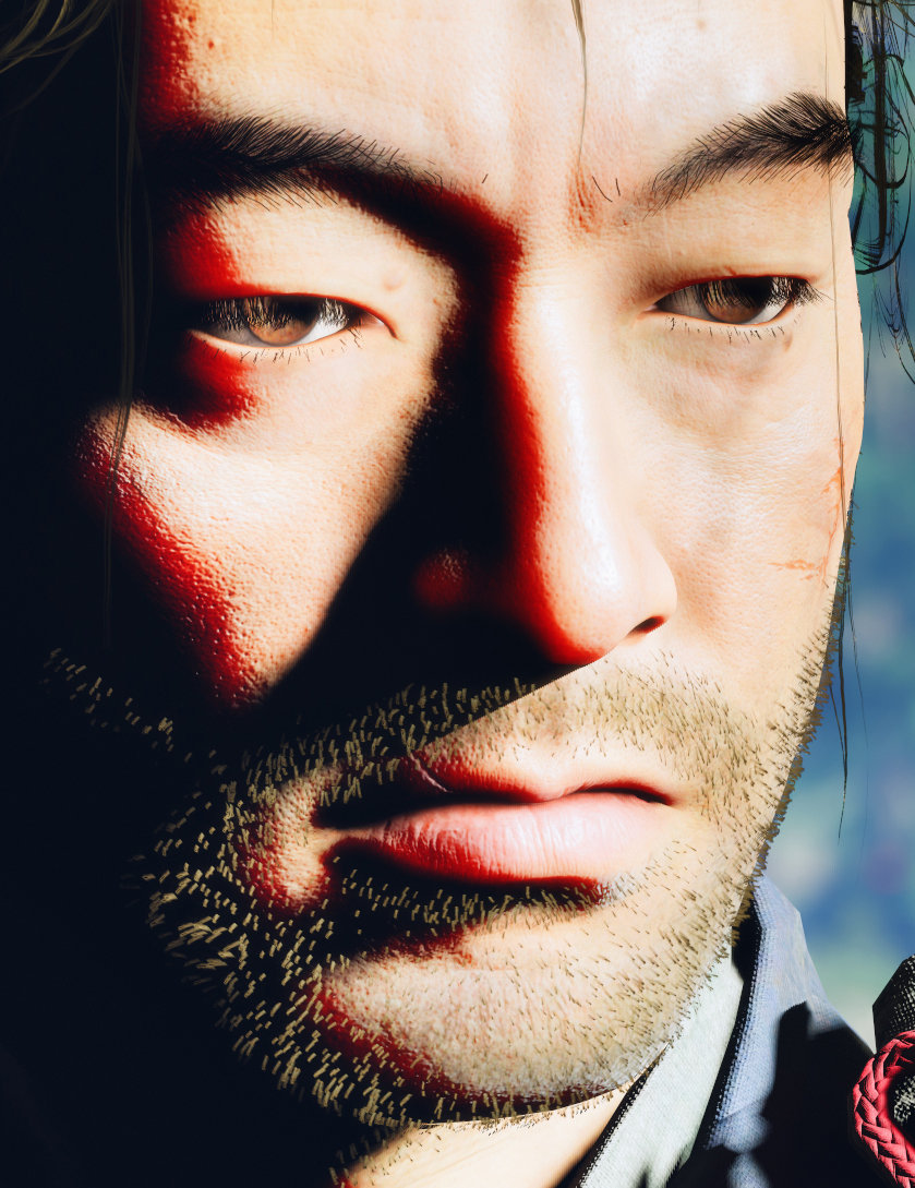
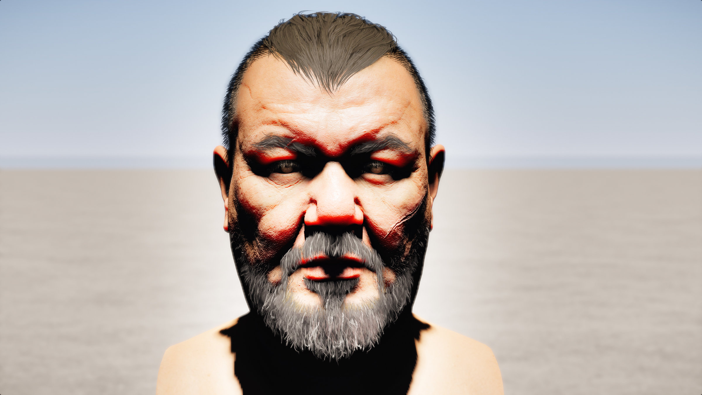
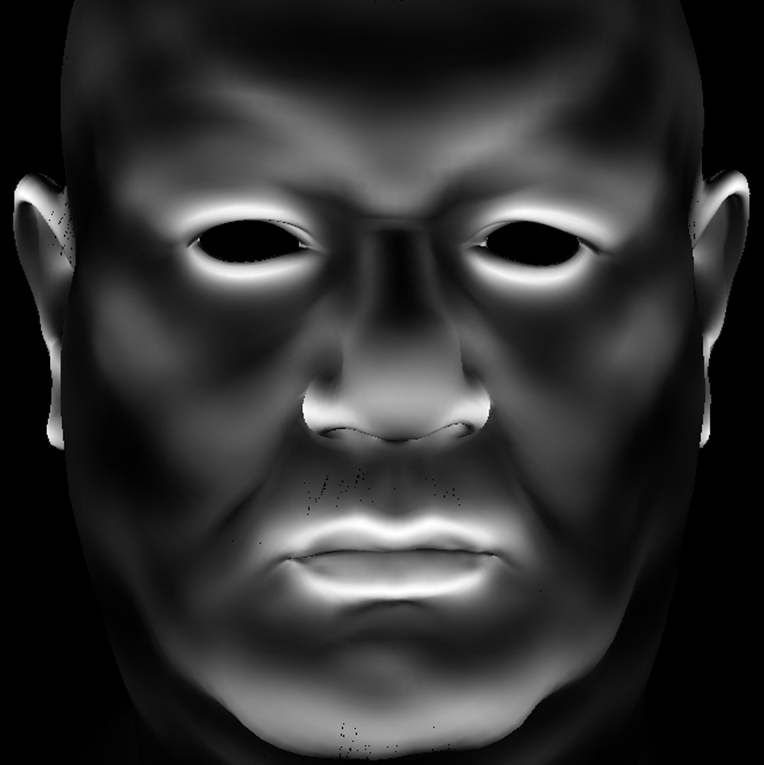
Skin Shading
Skin Shading
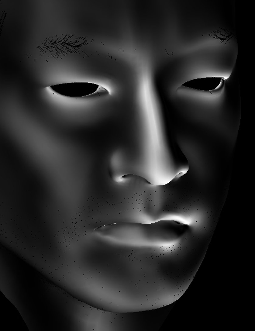
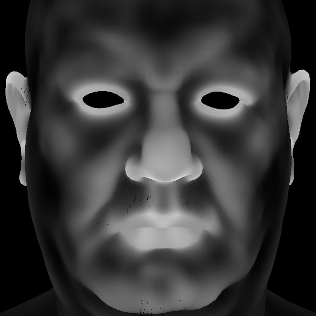
Skin Shading| Curvature

Skin Shading| Curvature

Skin Shading| Curvature
radial
linear
Skin Shading| Curvature
Skin Shading| Curvature
Skin Shading| Curvature
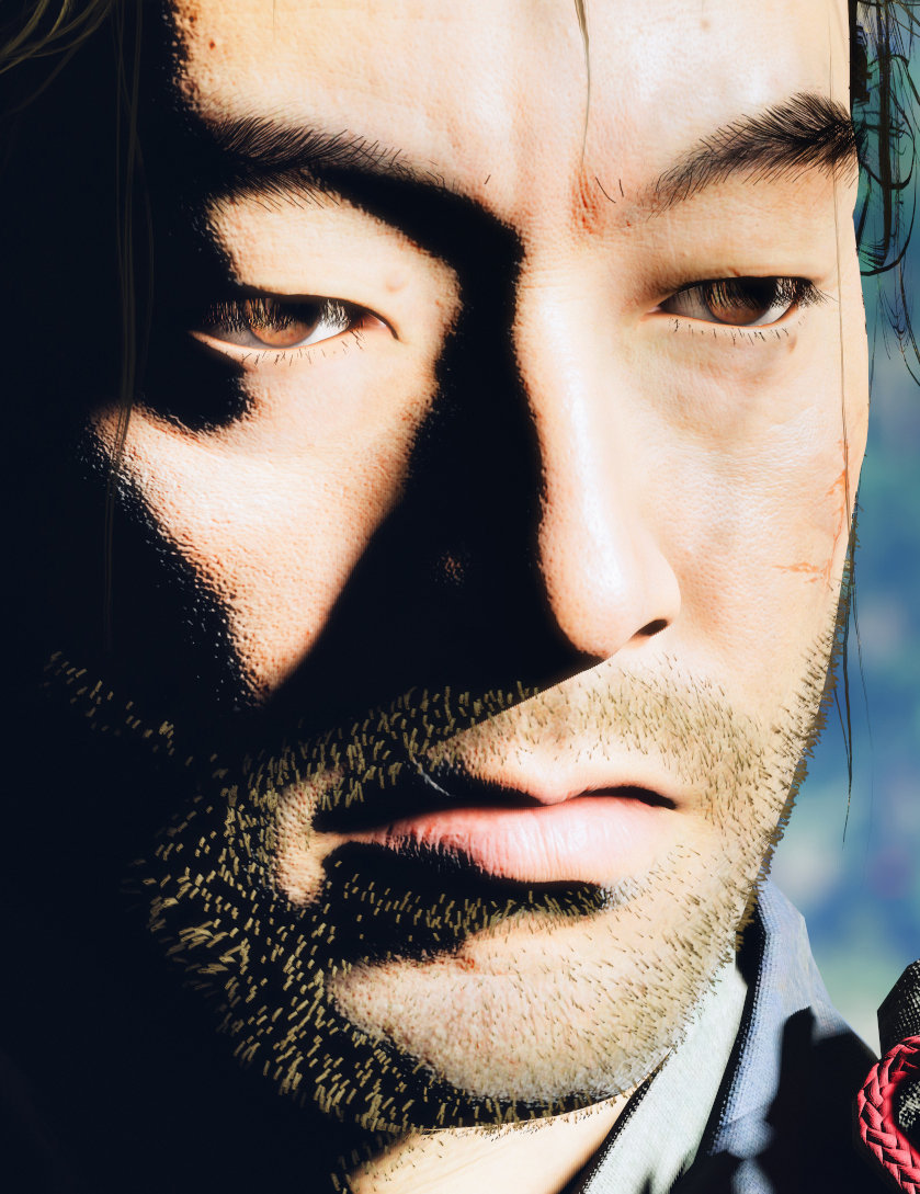
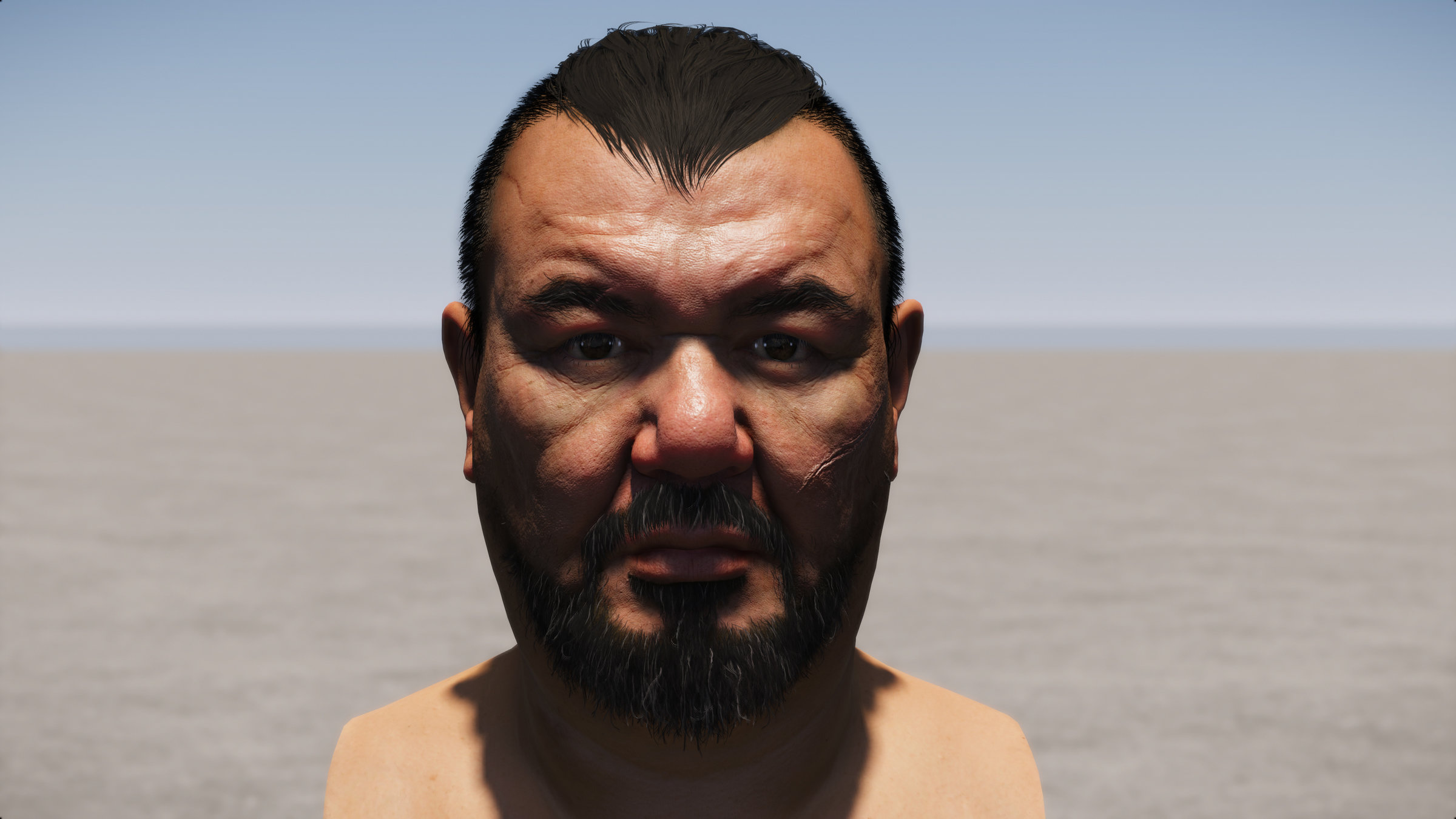
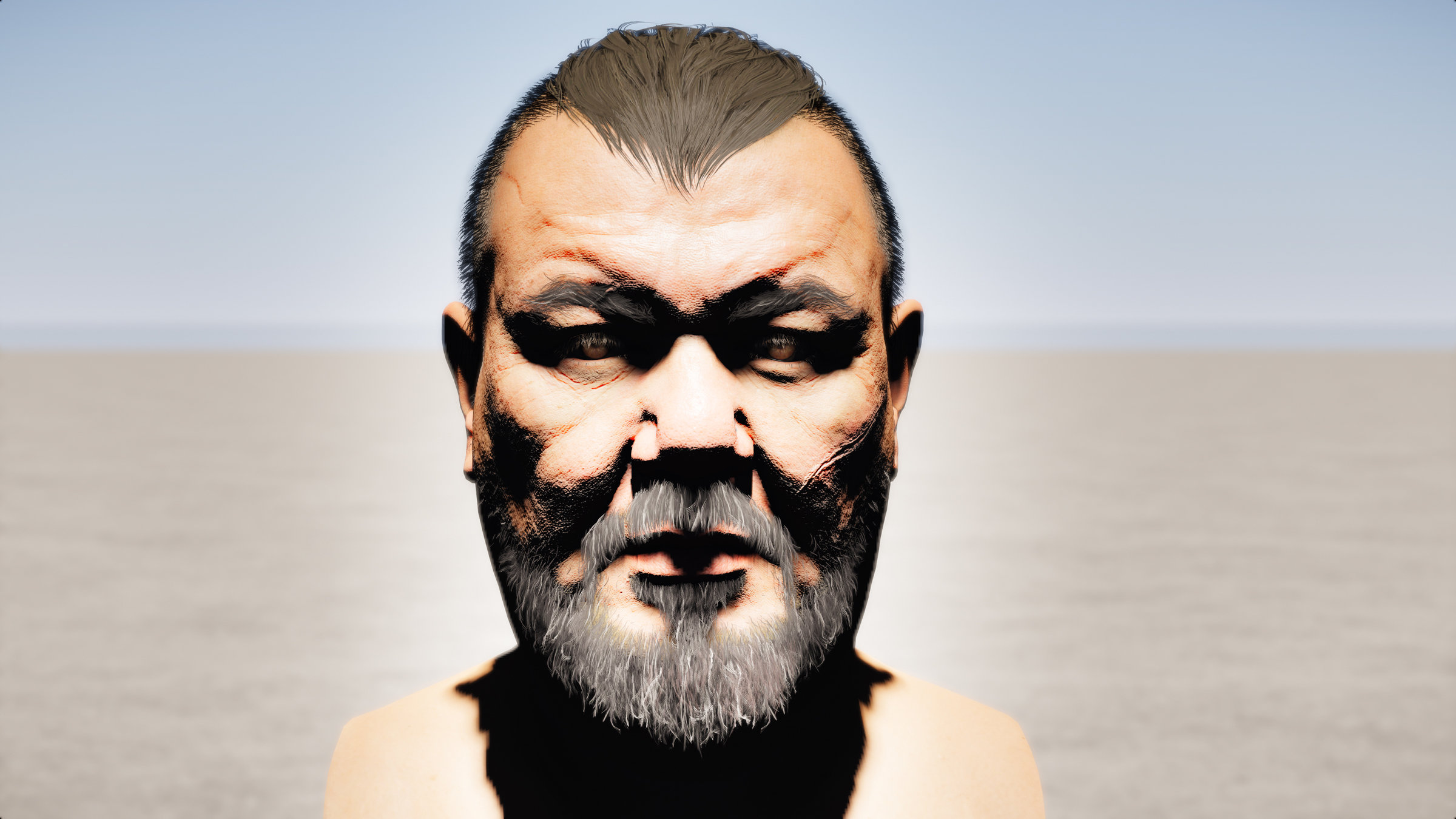
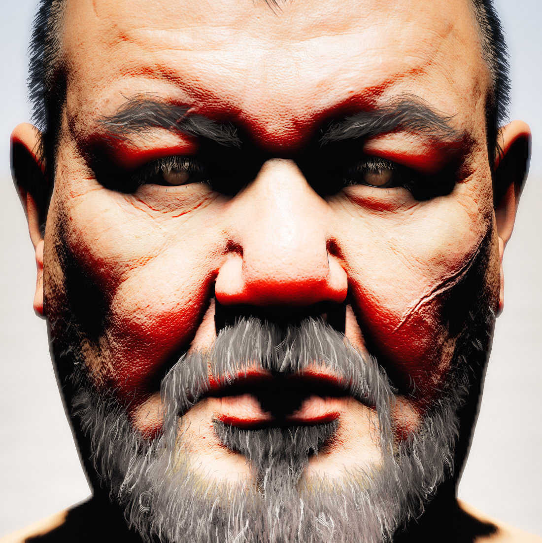
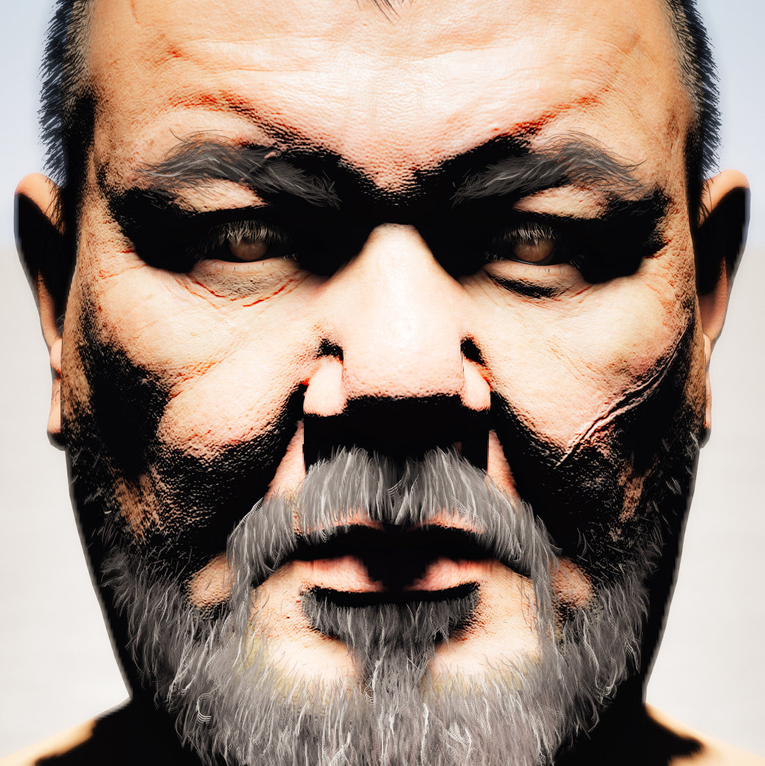
Skin Shading| Results
Zero Curvature

Mean Curvature

Directional Curvature

Zero Curvature
Mean Curvature
Directional Curvature
Mean Curvature
Directional Curvature
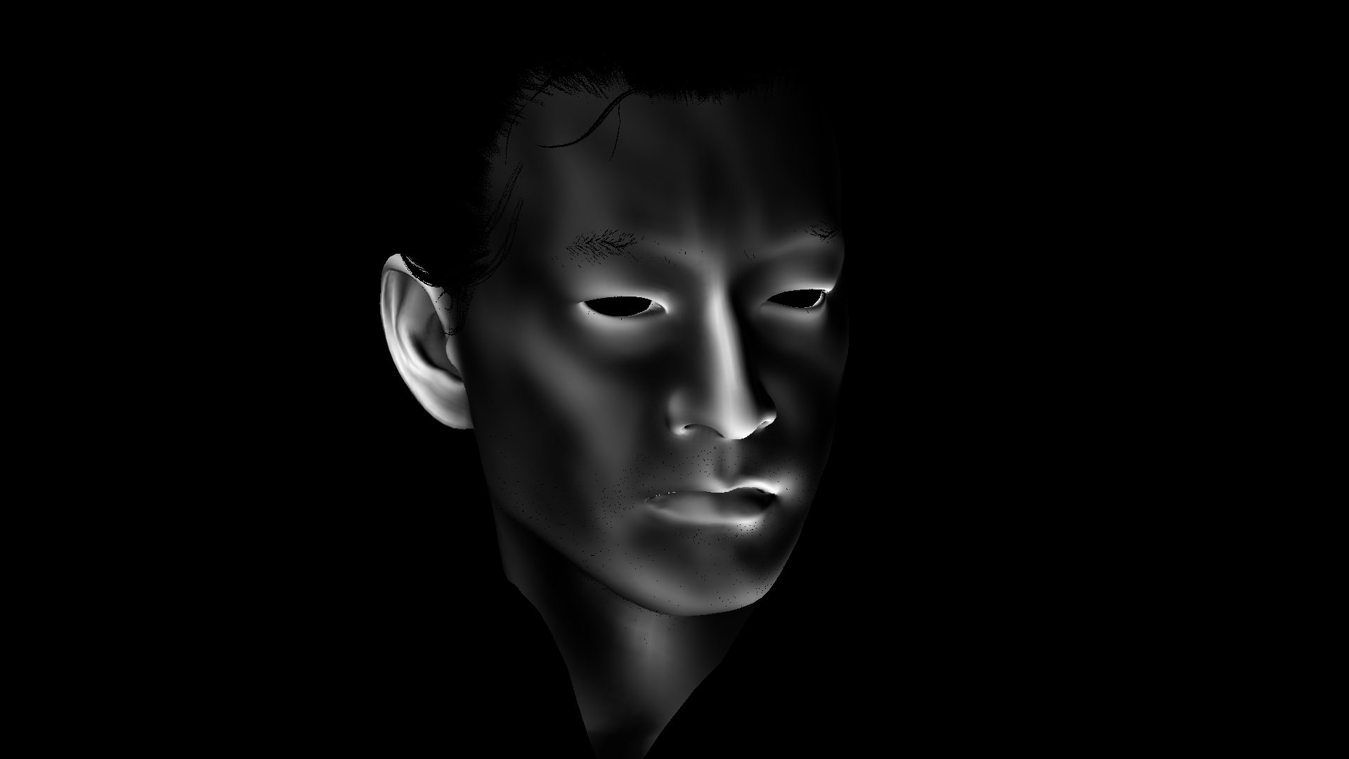
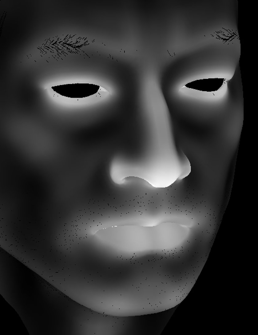
Zero Curvature
Mean Curvature
Directional Curvature

No Curvature

Mean Curvature

Directional Curvature
No Curvature
Mean Curvature

Directional Curvature
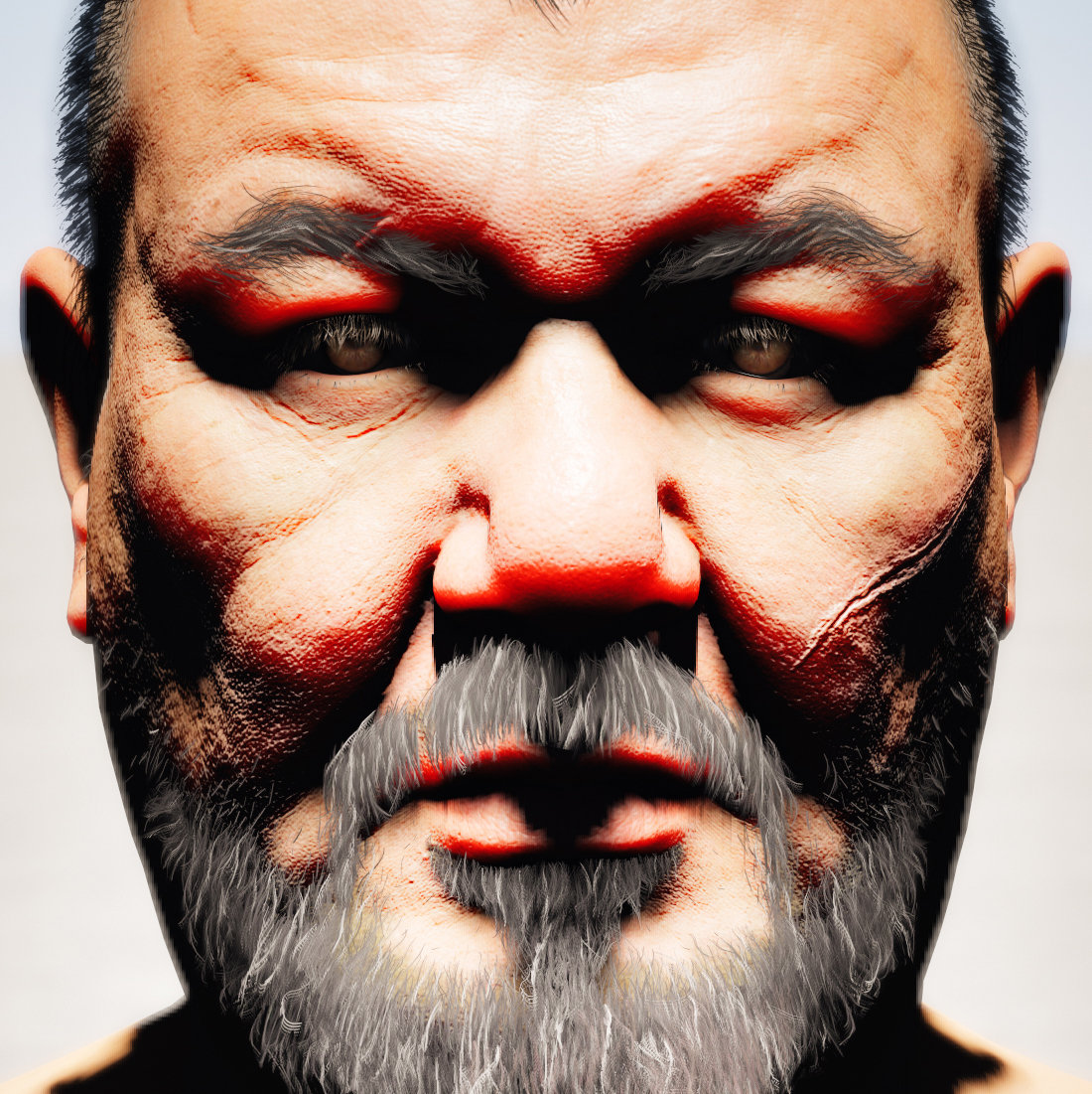
Zero Curvature
Mean Curvature
Directional Curvature

Skin Shading| Implementation
float CurvatureFromLight(
    float3 tangent,
    float3 bitangent,
    float3 curvTensor,
    float3 lightDir)
{
    // Project light vector into tangent plane

    float2 lightDirProj = float2(dot(lightDir, tangent), dot(lightDir, bitangent));

    // NOTE (jasminp) We should normalize lightDirProj here in order to correctly
    //    calculate curvature in the light direction projected to the tangent plane.
    //    However, it makes no perceptible difference, since the skin LUT does not vary
    //    much with curvature when N.L is large.

    float curvature = curvTensor.x * GSquare(lightDirProj.x) +
                        2.0f * curvTensor.y * lightDirProj.x * lightDirProj.y +
                        curvTensor.z * GSquare(lightDirProj.y);

    return curvature;
}
Skin Shading| Summary
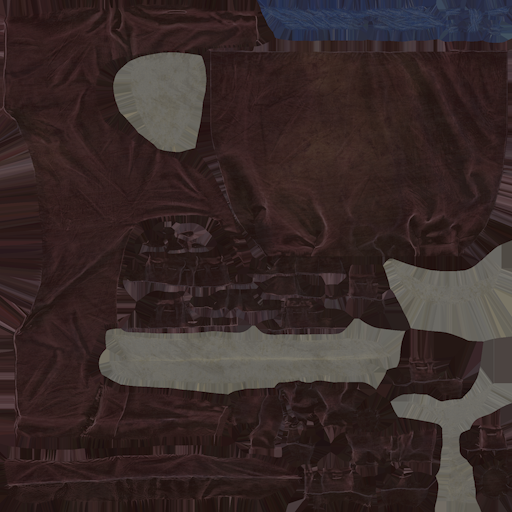
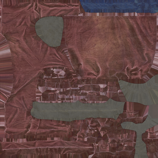
Detail Maps
Bonus Slide
Detail Maps
Bonus Slide
Detail Maps| Traditional Approach
Bonus Slide
Detail Maps| Our Approach
Bonus Slide
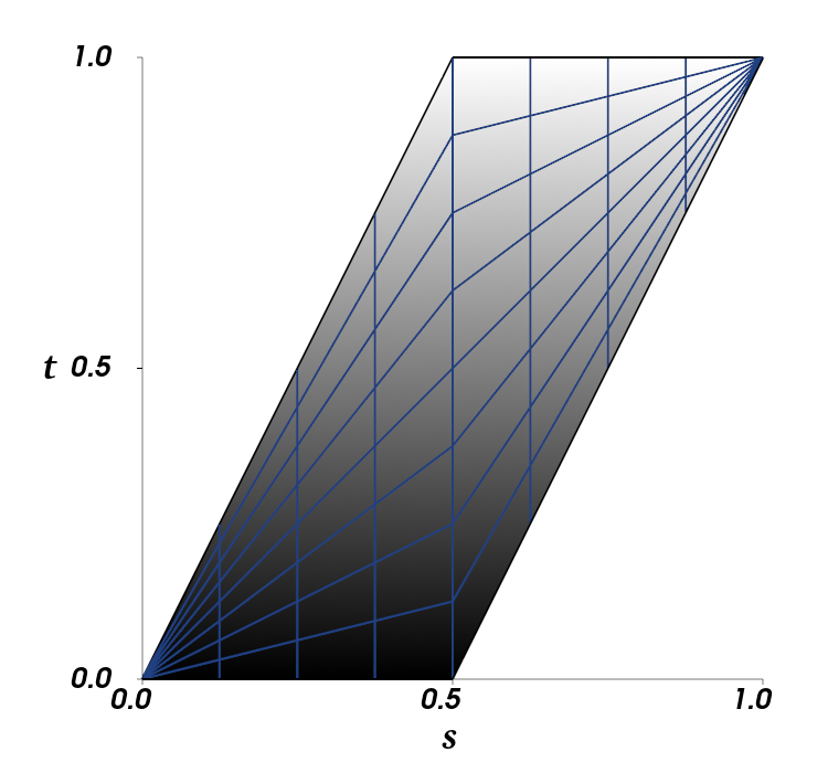
Detail Maps| Workflow
Bonus Slide
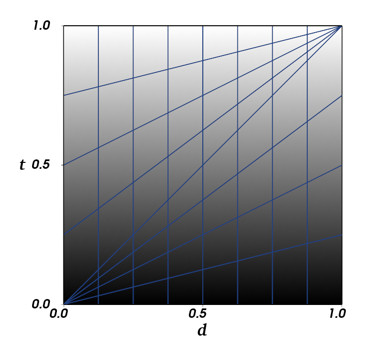
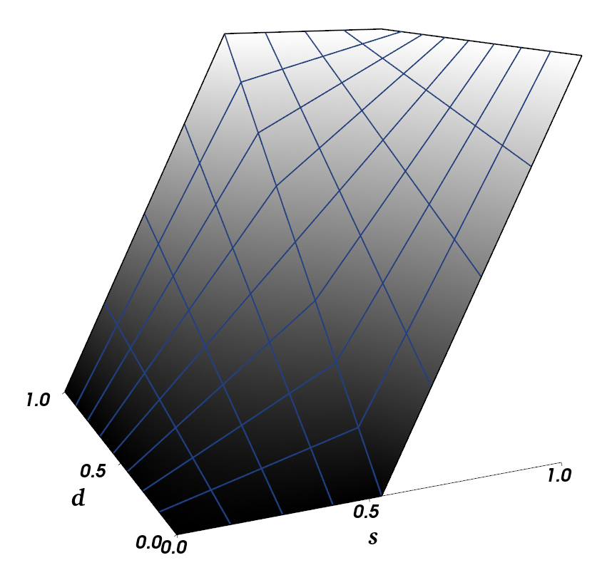
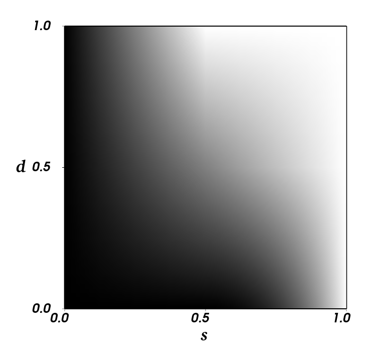
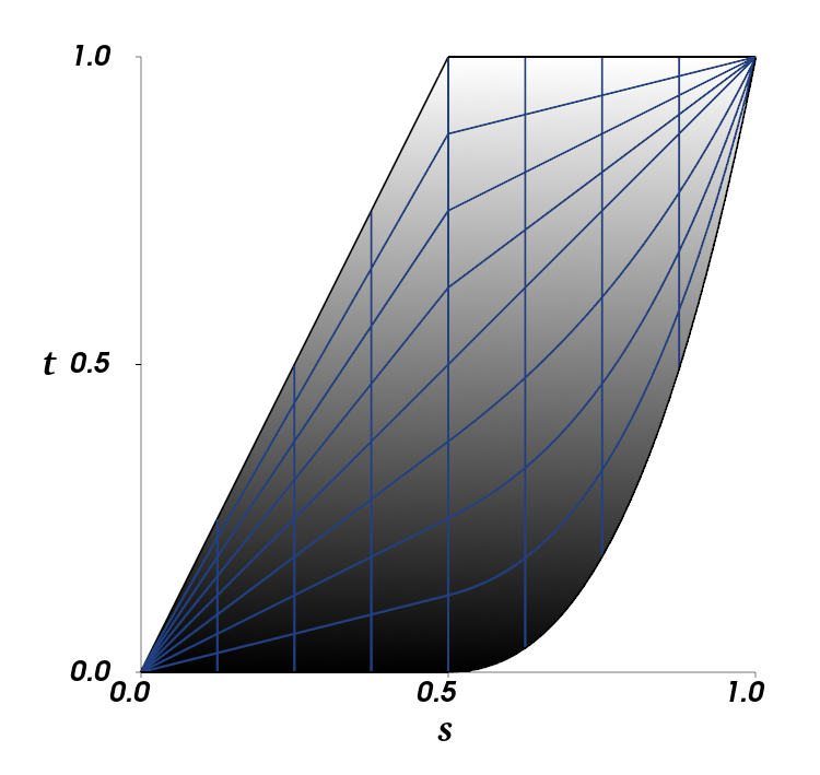
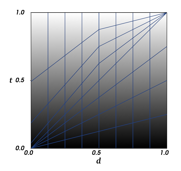
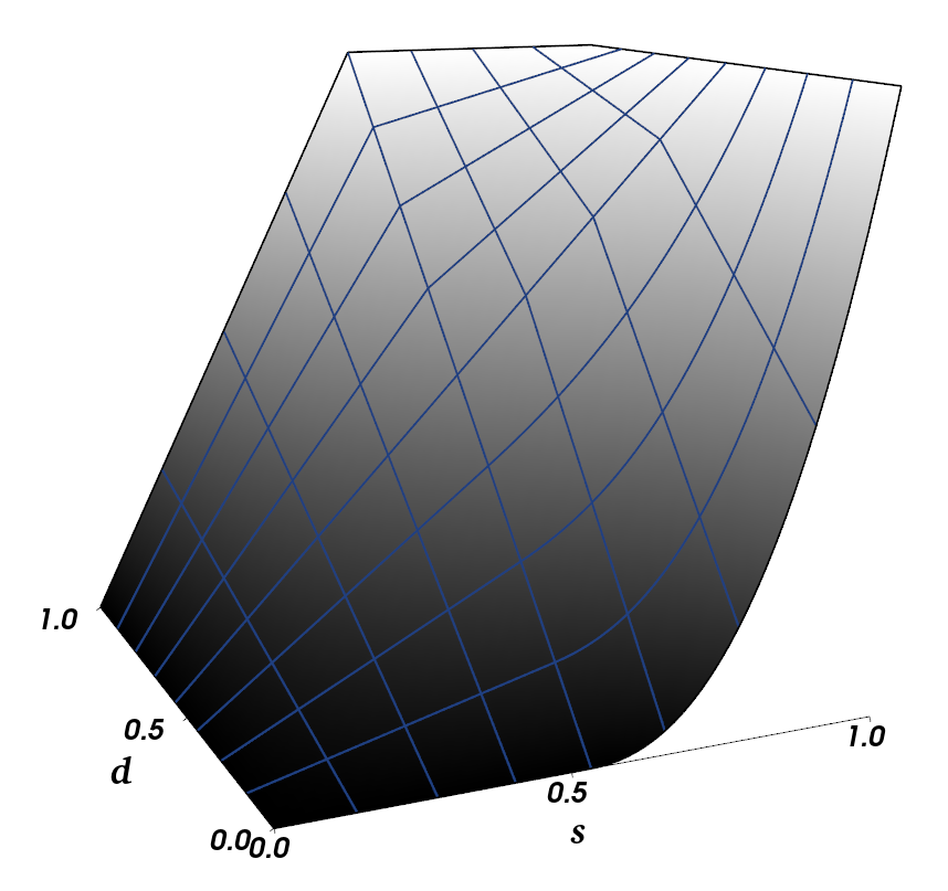
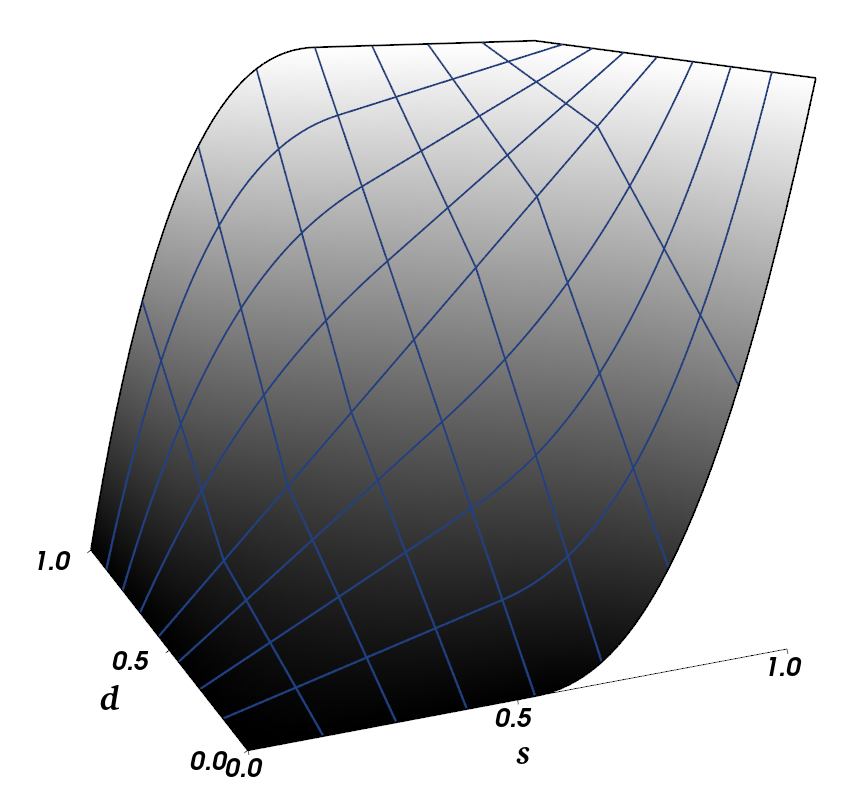
Detail Maps| Blending
Bonus Slide
Detail Maps| Blending
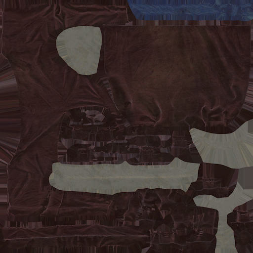
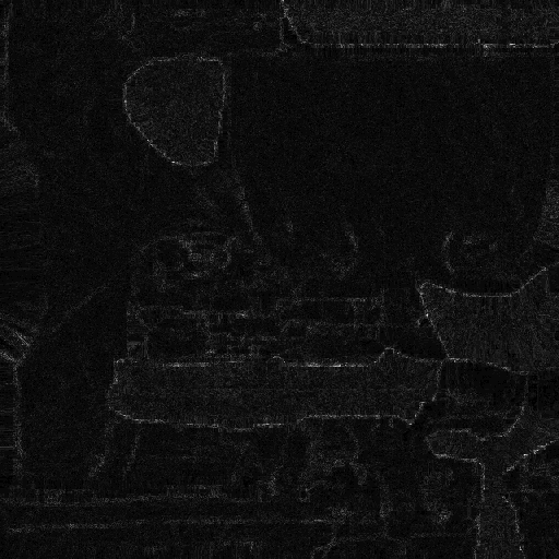
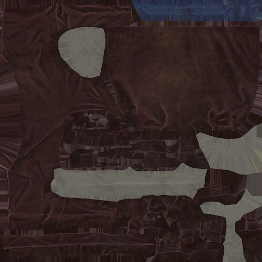
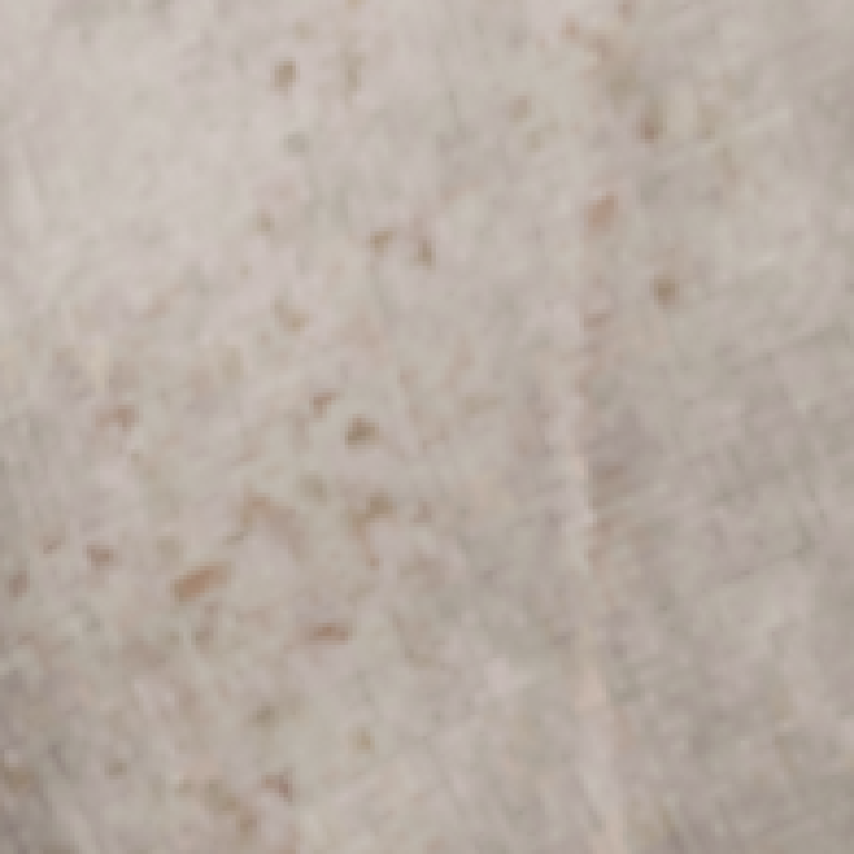
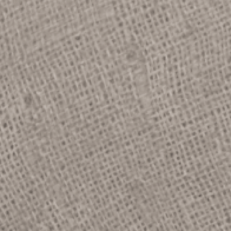
Synthesized
Detail
Target
Bonus Slide
Detail Maps| Blending
Bonus Slide
Detail Maps| Precision
Bonus Slide
Detail Maps| Precision
Bonus Slide
Detail Maps| Precision
Detail Maps| Precision
Bonus Slide
Detail Maps| Precision
Bonus Slide
Detail Maps| Precision
Bonus Slide
Detail Maps| Precision
No Detail
Bonus Slide
Detail Maps| Precision
Only Detail
Bonus Slide
Detail Maps| Precision
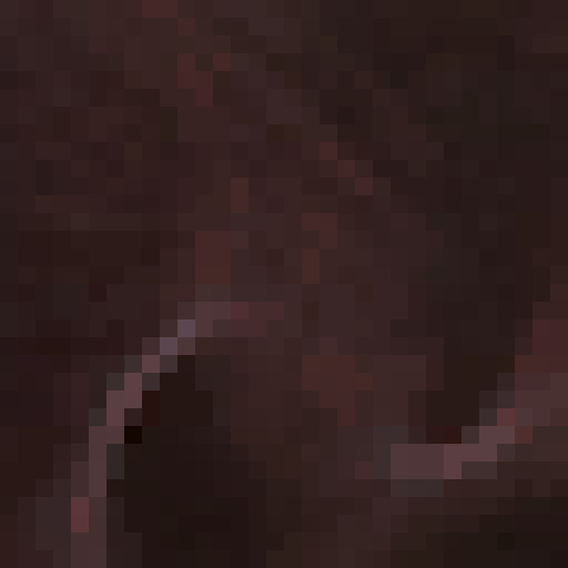
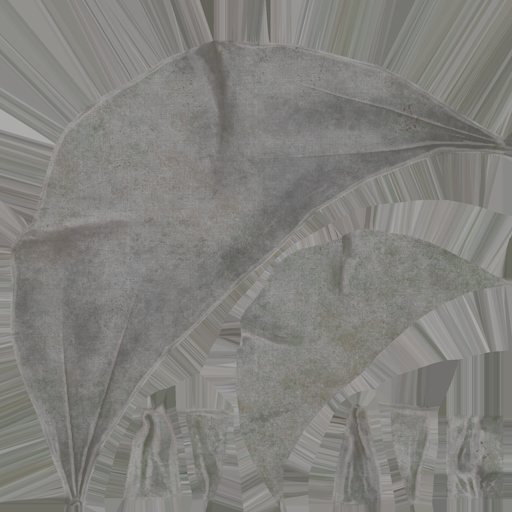
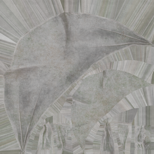
Synthesized
Detail
Target
Bonus Slide
Detail Maps| Precision
Target
Bonus Slide
Detail Maps| Precision
Target BC1
RMSE: 1.95
Bonus Slide
Detail Maps| Precision
Standard Overlay Blend
RMSE: 1.74
Bonus Slide
Detail Maps| Precision
Smooth Overlay Blend (Ours)
RMSE: 1.60
Bonus Slide
Detail Maps| Precision
Target BC1 Error
RMSE: 1.95
Bonus Slide
Detail Maps| Precision
Standard Overlay Blend Error
RMSE: 1.74
Bonus Slide
Detail Maps| Precision
Smooth Overlay Blend Error (Ours)
RMSE: 1.60
Bonus Slide
Detail Maps| Compression
Bonus Slide
Target
Detail Maps| Compression
Bonus Slide
Blend without Compression Compensation
Detail Maps| Compression
RMSE: 1.70
Bonus Slide
Blend with Compression Compensation (Ours)
Detail Maps| Compression
RMSE: 1.60
Bonus Slide
Error without Compression Compensation
Detail Maps| Compression
RMSE: 1.70
Bonus Slide
Error with Compression Compensation (Ours)
Detail Maps| Compression
RMSE: 1.60
Bonus Slide
Detail Maps| Compression
Bonus Slide
Detail Maps| Compression
Bonus Slide
Detail Maps| Compression
No Detail
Bonus Slide
Detail Maps| Compression
Only Detail
Bonus Slide
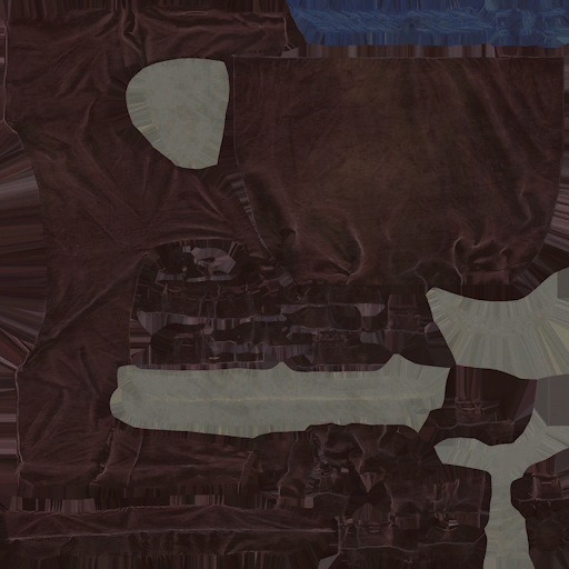
Synthesized
Detail
Target
Detail Maps| Compression
Bonus Slide
Target
Detail Maps| Compression
Bonus Slide
Blend without Compression Compensation
Detail Maps| Compression
RMSE: 2.43
Bonus Slide
Blend with Compression Compensation (Ours)
Detail Maps| Compression
RMSE: 2.00
Bonus Slide
Target
Detail Maps| Compression
Error without Compression Compensation
Detail Maps| Compression
RMSE: 2.43
Bonus Slide
Error with Compression Compensation (Ours)
Detail Maps| Compression
RMSE: 2.00
Bonus Slide


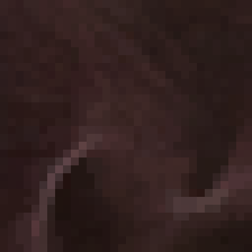
Synthesized
Detail
Target
Detail Maps| Compression
Target
Detail Maps| Compression
Blend without Compression Compensation
Detail Maps| Compression


PSNR: 39.53
Blend with Compression Compensation (Ours)
Detail Maps| Compression


PSNR: 43.55
Detail Maps| Statistics
Bonus Slide
Detail Maps| Other Blend Modes
Bonus Slide
Detail Maps | Summary
Bonus Slide
Acknowledgements
References