A Random Walk to the Ground Truth

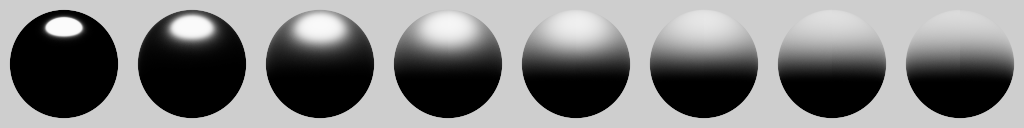
In the last post, we saw that significant energy was being lost due to the common single-scattering limitation of microfacet-based shading models:

An intuitive way to think about this is that these BRDFs are only modelling direct lighting (= single scattering) of the microsurface heightfield. Indirect lighting (= multiple scattering) is not simulated, and that is the cause of the missing energy in the image above.

So, why do we have this limitation? Well, in much the same way that direct lighting and shadowing is relatively straightforward to do in real-time compared to global illumination, the same is true for microfacet shading models.

Single scattering is solved efficiently by making certain simplifying assumptions about how microfacets of a microsurface are arranged. Through this, it’s possible to come up with analytic expressions for how light is directly reflected by the microsurface, while incorporating self shadowing.

This second aspect is modelled, naturally enough, by the shadowing term (part of the shadowing-masking term, $G$) of standard microfacet BRDFs. The Smith shadowing term [Smith 1976] is currently the most popular option here, and it has been shown by Heitz [2014] to produce results that are a close match to brute-force simulation. This is impressive considering that Smith’s model is pretty simple in terms of the microsurface assumptions that it makes.

Given the desirable properties of the Smith model (simple yet plausible, and also widely used), Heitz et al. [2016] chose to use it as the foundation for a new multiple-scattering model. It derives directly from Smith’s microsurface assumptions and is evaluated through a random walk process. As a result, all orders of scattering are accounted for, and energy conservation is achieved as a natural consequence.

Let’s return now to our earlier spheres, this time rendered using the Heitz model:

The rougher spheres are certainly a lot brighter than before, and placing them under uniform lighting (which matches the background) confirms that energy is now completely conserved:

Heitz et al. also showed that, just as with Smith and single-scattering, their multiple-scattering model has similar behaviour to a brute-force simulation. Given that property, I will proceed to use their model as a ground truth reference to compare Imageworks’ approach against.

$$ \newcommand{\fss }{\color{gray}{f_\mathrm{ss}}} \newcommand{\fms }{\color{purple}{f_\mathrm{ms}}} \newcommand{\Emo}{\color{olive}{E(\mu_o)}} \newcommand{\Emi}{\color{olive}{E(\mu_i)}} \newcommand{\Em }{\color{olive}{E(\mu)}} \newcommand{\Eavg}{\color{green}{E_\mathrm{avg}}} \newcommand{\Favg}{\color{teal}{F_\mathrm{avg}}} \newcommand{\Fms }{\color{brown}{F_\mathrm{ms}}} \newcommand{\FO }{F_0} \newcommand{\ki }{\color{}{k}} $$

A First Approximation

In contrast to the Heitz model, Imageworks’ solution is an approximation that attempts to compensate for the missing energy, rather than actually simulate the physical process of multiple scattering. This is achieved by adding an extra multiple-scattering lobe, $\fms$ – based on [Kelemen and Szirmay-Kalos 2001] – to the existing single-scattering BRDF, $\fss$:

$$ \begin{equation} f(\mu_o, \mu_i) = \fss\color{gray}{(\mu_o, \mu_i)} + \Fms \underbrace{\frac{(1 - \Emo)(1 - \Emi)}{\pi\,(1 - \Eavg)}}_{\fms \color{purple}{\text{: multiple scattering}}}. \label{eq:full_brdf} \end{equation} $$

Note: $\mu_o$ and $\mu_i$ are simply the view and light cosines, i.e. $n \cdot v$ and $n \cdot l$.

All of the details can be found in Kulla and Conty’s excellent presentation, but I’ll cover the salient points. Briefly, there are two terms that make up this additional Kelemen lobe:

• $\Em$: the directional albedo¹ of $\fss$ without Fresnel.
• $\Eavg$: the cosine-weighted average of $\Em$ over the hemisphere.

$\Emo$ is equivalent to what we saw previously with the furnace test result of a fully reflective, single-scattering material:

It’s the fraction of incoming light that leaves the microsurface after a single bounce, for the view angle $\mu_o$. The new lobe, $\fms$, is designed to account for the remainder, $1 - \Emo$, so that we get $\fss + \fms = 1$, i.e. perfect energy conservation.

For materials that aren’t 100% reflective, there’s a further term, $\Fms$, which I’ll discuss later. For now, let’s stick with our “fully reflective” assumption (in which case $\Fms = 1$) and examine the results of adding $\fms$:

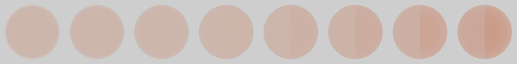
At first glance, the render looks pretty similar to the Heitz model, and we can see with a furnace test that energy is again conserved:

With a side-by-side comparison for each sphere (left half: Imageworks, right half: Heitz), we can see that indeed the two methods are very close, with only a minor visual difference at roughness = 1 (far right):

Here’s a zoomed in view of that particular case:

This is a promising early result, and I think you would be hard-pressed to tell the difference between the two in real production scenarios containing more complex lighting and spatially varying roughness, for instance.

Disorderly Conduct(or)

Now let’s see how things fare with more general conductors. To handle this case, Imageworks adapted a multiple-scattering Fresnel term, $\Fms$, from [Jakob et al. 2014] (Expanded Technical Report, Section 5.6), which accounts for absorption/tinting as light bounces multiple times on the microsurface:

$$ \begin{equation} \Fms = \frac{\Favg\,\Eavg}{1 - \Favg\,(1 - \Eavg)}, \label{eq:fms} \end{equation} $$

where $\Favg$ is the cosine-weighted average of the Fresnel function, $F$, over the hemisphere.

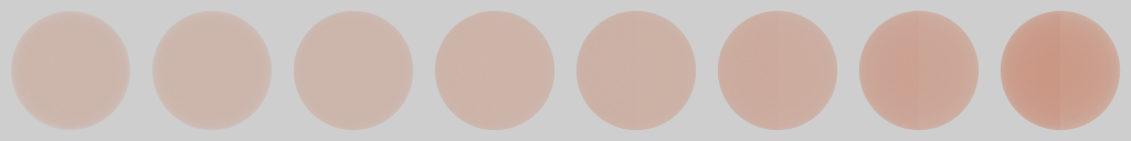
Here is a new side-by-side comparison (left half: Imageworks, right half: Heitz), with a copper material:

There’s now a bit more of a difference between the two approaches, which is easier to see in a furnace:

Evidently the Imageworks result is lighter and less saturated than Heitz at higher roughness.

When I first saw this difference, I was tempted to conclude that $\Fms$ is simply an approximation that fails to accurately model the complexities of real multiple scattering. However, a closer look at the derivation of this term revealed a problem.

The diffuse multiple-scattering model of Jakob et al. assumes that $\Eavg$ is the fraction of light that escapes the microsurface after each scattering event, leaving $1 - \Eavg$ to continue to bounce. Furthermore, each reflection is assumed to attenuate the light energy by $\Favg$. This means that after the first bounce, the fraction of light energy leaving the surface is $\Favg\,\Eavg$, followed by $\Favg\,\Eavg\,\Favg\,(1 - \Eavg)$, for the second bounce, etc. $\Fms$ is the total factor if we sum over all orders of scattering:

$$ \begin{align*} \Fms &= \Favg\,\Eavg + \Favg\,\Eavg\,\Favg\,(1 - \Eavg) + \Favg\,\Eavg\,\Favg^2\,(1 - \Eavg)^2 \ldots \\ &= \Favg\,\Eavg\,\sum_{\ki=0}^{\infty}\Favg^{\ki}\,(1 - \Eavg)^{\ki} \\ &= \frac{\Favg\,\Eavg}{1 - \Favg\,(1 - \Eavg)}. \end{align*} $$

Note: this is equivalent to the interreflection model of Stewart and Langer [1996] (Equation 2).²

The problem is that this model is including single scattering events ($\Favg\,\Eavg$), which we’ve already accounted for with $\fss$. This suggests that we should instead use:

$$ \begin{align*} \Fms &= \Favg\,\Eavg\,\sum_{\ki=1}^{\infty}\Favg^{\ki}\,(1 - \Eavg)^{\ki} \\ &= \frac{\Favg^2\,\Eavg\,(1 - \Eavg)}{1 - \Favg\,(1 - \Eavg)}. \end{align*} $$

However, this now gives $\Fms = 1 - \Eavg$ when $\Favg = 1$, instead of $\Fms = 1$ previously. We want the latter behaviour because the $\fms$ lobe already has a magnitude of $1 - \Emo$ (as discussed earlier), so we should normalise our adjusted $\Fms$ by $1/(1 - \Eavg)$:

$$ \begin{equation} \Fms = \frac{\Favg^2\,\Eavg}{1 - \Favg\,(1 - \Eavg)}. \end{equation} $$

This is very close to what we had before (Eq. $\ref{eq:fms}$), except there’s $\Favg^2$ instead of $\Favg$ in the numerator.

With this simple change, the Imageworks solution gets closer to the ground truth:

The furnace test reveals that there is still a small difference: Imageworks is now a bit darker and more saturated compared to Heitz. Still, it’s an overall improvement.

This adjustment has been added to an updated version of Imageworks’ slides, along with numerical fits for $\Em$ and $\Eavg$ from Christopher Kulla. The new slides also contain several important corrections³ that are highlighted in the speaker notes.

In the next post, I discuss a further improvement to $\Fms$ that gets us even closer to the reference.