
|
+ | 
|
= | 
|
| By Colin Barré-Brisebois and Stephen Hill. | ||||
The x, why, z
It’s a seemly simple problem: given two normal maps, how do you combine them? In particular, how do you add detail to a base normal map in a consistent way? We’ll be examining several popular methods as well as covering a new approach, Reoriented Normal Mapping, that does things a little differently.
This isn’t an exhaustive survey with all the answers, but hopefully we’ll encourage you to re-examine what you’re currently doing, whether it’s at run time or in the creation process itself.
Does it Blend?
Texture blending crops up time and again in video game rendering. Common uses include: transitioning between materials, breaking up tiling patterns, simulating local deformation through wrinkle maps, and adding micro details to surfaces. We’ll be focusing on the last scenario here.
The exact method of blending depends on the context; for albedo maps, linear interpolation typically makes sense, but normal maps are a different story. Since the data represents directions, we can’t simply treat the channels independently as we do for colours. Sometimes this is disregarded for speed or convenience, but doing so can lead to poor results.
Linear Blending
To see this in action, let’s take look at a simple case of adding high-frequency detail to a base normal map (a cone) in a naive way:
|
|
+ |
|
= | 
|
Here we’re just unpacking the normal maps, adding them together, renormalising and finally repacking for visualisation purposes:
1float3 n1 = tex2D(texBase,   uv).xyz*2 - 1;
2float3 n2 = tex2D(texDetail, uv).xyz*2 - 1;
3float3 r  = normalize(n1 + n2);
4return r*0.5 + 0.5;
The output is similar to averaging, and because the textures are quite different, we end up ‘flattening’ both the base orientations and the details. This leads to unintuitive behaviour even in simple situations such as when one of the inputs is flat: we expect it to have no effect, but instead we get a shift towards $[0, 0, 1]$.
Overlay Blending
A common alternative on the art side is the Overlay blend mode:
|
|
+ |
|
= | 
|
Here’s the reference code:
1float3 n1 = tex2D(texBase,   uv).xyz;
2float3 n2 = tex2D(texDetail, uv).xyz;
3float3 r  = n1 < 0.5 ? 2*n1*n2 : 1 - 2*(1 - n1)*(1 - n2);
4r = normalize(r*2 - 1);
5return r*0.5 + 0.5;
While there does appear to be an overall improvement, the combined normals still look incorrect. That’s hardly surprising though, because we’re still processing the channels independently! In fact there’s no rationale for using Overlay except that it tends to behave a little better than the other Photoshop blend modes, which is why it’s favoured by some artists.
Partial Derivative Blending
Things would be a lot more sane if we could work with height instead of normal maps, since standard operations would function predictably. Sadly, height maps are not always available during the creation process, and can be impractical to use directly for shading.
Fortunately, equivalent results can be achieved by using the partial derivatives (PDs) instead, which are trivially computed from the normal maps themselves. We won’t go into the theory here, since Jörn Loviscach has already covered the topic in some depth [1]. Instead, let’s go right ahead and apply this approach to the problem at hand:
|
|
+ |
|
= | 
|
Again, here’s some reference code:
1float3 n1 = tex2D(texBase,   uv).xyz*2 - 1;
2float3 n2 = tex2D(texDetail, uv).xyz*2 - 1;
3float2 pd = n1.xy/n1.z + n2.xy/n2.z; // Add the PDs
4float3 r  = normalize(float3(pd, 1));
5return r*0.5 + 0.5;
In practice, the 3rd and 4th lines should be replaced with the following for robustness:
1float3 r = normalize(float3(n1.xy*n2.z + n2.xy*n1.z, n1.z*n2.z));Looking at Figure 3, the output is clearly much better than before. The combined map now resembles a perturbed version of the base, as one would expect. By simply adding the partial derivatives together, the flat normal case is handled correctly as well.
Alas, the process isn’t perfect, because detail remains subdued over the surface of the cone. That said, it does work well when used to fade between materials instead (see [1] or [2] for examples):
1float2 pd = lerp(n1.xy/n1.z, n2.xy/n2.z, blend);
2float3 r = normalize(float3(pd, 1));
Whiteout Blending
At SIGGRAPH'07, Christopher Oat described the approach used by the AMD Ruby: Whiteout demo [3] for the purpose of adding wrinkles:
|
|
+ |
|
= | 
|
The code looks a lot like the PD one in its second form, except that there’s no scaling by z for the xy components:
1float3 r = normalize(float3(n1.xy + n2.xy, n1.z*n2.z));With this modification, detail is more apparent over the cone, while flat normals still act intuitively.
UDN Blending
Finally, an even simpler form appears on the Unreal Developer Network [4].
|
|
+ |
|
= | 
|
The only change from the last technique is that it drops the multiplication by n2.z:
1float3 r = normalize(float3(n1.xy + n2.xy, n1.z));Another way to view this is that it’s linear blending, except that we only add $x$ and $y$ from the detail map.
As we’ll see later, this can save some shader instructions over Whiteout, which is always useful for lower-end platforms. However, it also leads to some detail reduction over flatter base normals – see the corners of the output for the worst case – although this may go unnoticed. In fact, on the whole, the visual difference over Whiteout is hard to detect here. See Figure 5 in the next section for a better visual comparison.
Detail Oriented
Now for our own method. We were looking for the following properties in order to provide intuitive behaviour to artists:
- Logical: the operation has a clear mathematical basis (e.g. geometric interpretation)
- Handles identity: if one of the normal maps is flat, the output matches the other normal map
- No flattening: the strength of both normal maps is preserved
Although the Whiteout solution appears to work well, it’s a bit fuzzy on the first and last points.
To meet these goals, our strategy involves rotating (or reorienting) the detail map so that it follows the ‘surface’ of the base normal map, just as tangent-space normals are transformed by the underlying geometry when lighting in object or world space. We’ll refer to this as Reoriented Normal Mapping (RNM). Here’s the result compared to the last two techniques:

The difference in detail is noticeable, and this shows through in the final shading (see demos at the end).
To be clear, we’re not the only ones to think of this. Essentially the same idea – developed for adding pores to skin as part of a Unity tech demo – was recently presented at GDC by Renaldas Zioma [5]. There are probably earlier examples too, although we’ve struggled to find any so far. That said, there are some advantages to our approach over the Unity one, as we’ll explain once we’ve dived into the implementation.
The Nitty Gritty
Okay, brace yourself for some maths. Let’s say that we have a geometric normal $\mathbf{s}$, a base normal $\mathbf{t}$ and a secondary (or detail) normal $\mathbf{u}$. We can compute the reoriented normal $\mathbf{r}$ by building a transform that rotates $\mathbf{s}$ onto $\mathbf{t}$, then applying this to $\mathbf{u}$:
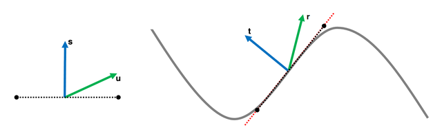
Figure 7: Reorienting a detail normal u (left) so it follows the base normal map (right).
We can achieve this transform via the shortest arc quaternion [6]:
$$ \begin{equation} \mathbf{\hat{q}} = \left[\mathbf{q}_{v}, q_{w}\right] = \frac{1}{\sqrt{2(\mathbf{s} \cdot \mathbf{t} + 1)}} \left[\mathbf{s} \times \mathbf{t}, \mathbf{s} \cdot \mathbf{t} + 1 \right] \label{eq:quat} \end{equation} $$The rotation of $\mathbf{u}$ can then be performed in the standard way [7]:
$$ \begin{alignat}{2} \mathbf{r} = \mathbf{\hat{q}}\mathbf{\hat{p}}\mathbf{\hat{q}^{*}}, ~\mbox{where}~~ &\mathbf{\hat{q}^{*}} &=& \left[-\mathbf{q}_{v}, q_{w}\right]\\\\ &\mathbf{\hat{p}} &=& \left[\mathbf{u}, 0\right]\nonumber \end{alignat} $$As shown by [8], this reduces to:
$$ \begin{equation} \mathbf{r} = \mathbf{u}(q_w^2 - \mathbf{q}_v \cdot \mathbf{q}_v) + 2\mathbf{q}_v(\mathbf{q}_v \cdot \mathbf{u}) + 2q_w(\mathbf{q}_v \times \mathbf{u})\label{eq:rotation} \end{equation} $$Since we are operating in tangent space, by convention $\mathbf{s} = \left[0, 0, 1\right]$. Consequently, if we substitute $\eqref{eq:quat}$ into $\eqref{eq:rotation}$ and simplify, we obtain:
$$ \begin{alignat}{2} \mathbf{r} = 2\mathbf{q}(\mathbf{q} \,\cdot\, \mathbf{u}')\,-\, \mathbf{u}', ~\mbox{where}~~ &\mathbf{q} &=& \frac{1}{\sqrt{2(t_z + 1)}}\left[t_x, t_y, t_z + 1\right]\label{eq:simplified}\\\\ &\mathbf{u}' &=& \left[-u_x, -u_y, u_z\right]\nonumber \end{alignat} $$Which further reduces to:
$$ \begin{equation} \mathbf{r} = \frac{\mathbf{t}'}{t'_z}(\mathbf{t}'\cdot \mathbf{u}') - \mathbf{u}', ~\mbox{where}~~ \mathbf{t}' = \left[t_x, t_y, t_z + 1\right]\label{eq:final} \end{equation} $$Here is the HLSL implementation of $\eqref{eq:final}$, with additions and sign changes folded into the unpacking of the normals. For convenience, u and t are $\mathbf{t}’$ and $\mathbf{u}’$ above:
1float3 t = tex2D(texBase,   uv).xyz*float3( 2,  2, 2) + float3(-1, -1,  0);
2float3 u = tex2D(texDetail, uv).xyz*float3(-2, -2, 2) + float3( 1,  1, -1);
3float3 r = t*dot(t, u)/t.z - u;
4return r*0.5 + 0.5;
A potentially neat property of this method is that the length of $\mathbf{u}$ is preserved if $\mathbf{t}$ is unit length, so if $\mathbf{u}$ is also unit length then no normalisation is required! However, this is unlikely to hold true in practice due to quantisation, compression, mipmapping and filtering. You may not see a significant impact on diffuse shading, but it can really affect energy-conserving specular. Given that, we recommend normalising the result:
1float3 r = normalize(t*dot(t, u) - u*t.z);Devil in the Details
Whilst we were preparing this article, we learned of an upcoming paper by Jeppe Revall Frisvad [9] that uses the same strategy for rotating a local vector. Here’s the relevant code adapted to HLSL:
 1float3 n1 = tex2D(texBase,   uv).xyz*2 - 1;
 2float3 n2 = tex2D(texDetail, uv).xyz*2 - 1;
 3
 4float a = 1/(1 + n1.z);
 5float b = -n1.x*n1.y*a;
 6
 7// Form a basis
 8float3 b1 = float3(1 - n1.x*n1.x*a, b, -n1.x);
 9float3 b2 = float3(b, 1 - n1.y*n1.y*a, -n1.y);
10float3 b3 = n1;
11
12if (n1.z < -0.9999999) // Handle the singularity
13{
14    b1 = float3( 0, -1, 0);
15    b2 = float3(-1,  0, 0);
16}
17
18// Rotate n2 via the basis
19float3 r = n2.x*b1 + n2.y*b2 + n2.z*b3;
20
21return r*0.5 + 0.5;
Our version is written with GPUs in mind and requires less ALU operations in this context, whereas Jeppe’s implementation is appropriate for situations where the basis can be reused, such as Monte Carlo sampling. Another thing to note is that there’s a singularity when the $z$ component of the base normal is $-1$. Jeppe checks for this, but in our case we can guard against it within the art pipeline instead.
More importantly, we could argue that $z$ should be $\geq 0$, but this is not always true of the output of our method! One potential issue is if reorientation is used during authoring, followed by compression to a two-component normal map format, since reconstruction normally assumes that $z$ is $\geq 0$. The most straightforward fix is to clamp $z$ to $0$ and renormalise prior to compression.
As for shading, we haven’t seen any adverse affects from negative $z$ values – i.e., where the reoriented normal points into the surface – but this is certainly something to bear in mind. We’re interested in hearing your experiences.
Unity Blending
Let’s return now to the approach taken for the Unity tech demo. Like Jeppe, Renaldas also uses a basis to transform the secondary normal. This is created by rotating the base normal around the $y$ and $x$ axes to generate the other two rows of the matrix:
 1float3 n1 = tex2D(texBase,   uv).xyz*2 - 1;
 2float3 n2 = tex2D(texDetail, uv).xyz*2 - 1;
 3
 4float3x3 nBasis = float3x3(
 5    float3(n1.z, n1.y, -n1.x), // +90 degree rotation around y axis
 6    float3(n1.x, n1.z, -n1.y), // -90 degree rotation around x axis
 7    float3(n1.x, n1.y,  n1.z));
 8
 9float3 r = normalize(n2.x*nBasis[0] + n2.y*nBasis[1] + n2.z*nBasis[2]);
10return r*0.5 + 0.5;
Note: This code differs slightly from the version in the “Mastering DirectX 11 with Unity” slides. The first row of the basis has been corrected.
However, the basis is only othonormal when n1 is $[0,0,\pm1]$ and things progressively degenerate the further the normal drifts from either of these two directions. As a visual example, Figure 8 shows what happens as we rotate n1 towards the $x$ axis and transform a set of points on the upper hemisphere ($+z$) in place of n2:
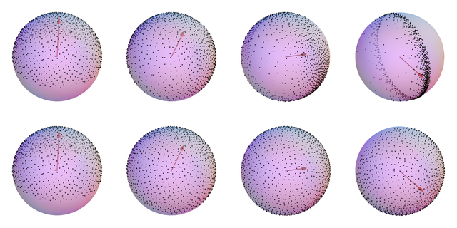
Figure 8: Unity basis (top row) vs quaternion transform (bottom row).
With Unity, the points collapse to a circle as n1 reaches the $x$ axis because the basis goes to:
In contrast, there’s no such issue for the quaternion transform. This is also reflected in the blended output:
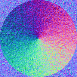
|
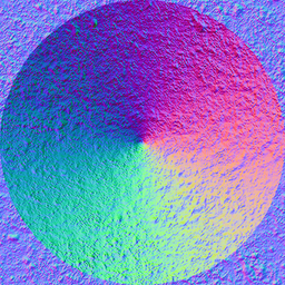
|
Start Your Engines
Giving representative performance figures is an impossible task, as it very much depends on a number of factors: the platform, surrounding code, choice of normal map encoding (which might be unique to your game), and possibly even the shader compiler.
As a guide, we’ve taken the core of the various techniques – minus texture reads and repacking – and optimised them for the Shader Model 3.0 virtual instruction set (see Appendix). Here’s how they fare in terms of instruction count:
| Method | SM3.0 ALU Inst. |
| Linear | 5 |
| Overlay | 9 |
| PD | 7 |
| Whiteout | 7 |
| UDN | 5 |
| RNM * | 8 |
| Unity | 8 |
* This includes normalisation. If it turns out that you don’t need it, then RNM is 6 ALU instructions.
In reality the GPU may be able to pair some instructions, and certain operations could be more expensive than others. In particular, normalize expands to dot rcp mul here, but a certain console provides a single instruction nrm at half precision.
For space (and time!), we haven’t included code and stats for two-component normal map encodings, but the $z$ reconstruction should be similar for most methods. One exception is with UDN, since the $z$ component of the detail normal isn’t used, making the technique particularly attractive in this case.
A Light Demo
By now, I’m sure you’re wondering how these methods compare under lighting, so here is a simple WebGL demo with a moving light source. We’ve also put together a RenderMonkey project, so you can easily test things out with your own textures.
Conclusions
Based on the analysis and results, it’s clear to us that Linear and Overlay blending have no redeeming value when it comes to detail normal mapping. Even when GPU cycles are at a premium, UDN represents a better option, and it should be easy to replicate in Photoshop as well.
Whether you see any benefit from Whiteout over UDN could depend on your textures and shading model – in our example, there’s very little separating them. Beyond these, RNM can make a difference in terms of retaining more detail, and at a similar instruction cost, so we hope you find it a compelling alternative.
In addition to two component formats, we also haven’t covered fading strategies, integration with parallax mapping, or specular anti-aliasing. These are topics we’d like to address in the future.
Acknowledgements
Firstly, credit should be given to Gabriel Lassonde for the initial idea of rotating normals using quaternions for the purpose of blending. Secondly, would like to thank Pierric Gimmig, Steve McAuley and Morgan McGuire for helpful comments, plus David Massicotte for creating the example normal maps.
References
[1] Loviscach, J., “Care and Feeding of Normal Vectors”, ShaderX^6, Charles River Media, 2008.
[2] Mikkelsen, M., “How to do more generic mixing of derivative maps?”, 2012.
[3] Oat, C., “Real-Time Wrinkles”, Advanced Real-Time Rendering in 3D Graphics and Games, SIGGRAPH Course, 2007.
[4] “Material Basics: Detail Normal Map”, Unreal Developer Network.
[5] Zioma, R., Green, S., “Mastering DirectX 11 with Unity”, GDC 2012.
[6] Melax, S., “The Shortest Arc Quaternion”, Game Programming Gems, Charles River Media, 2000.
[7] Akenine-Möller, T., Haines, E., Hoffman, N., Real-Time Rendering 3rd Edition, A. K. Peters, Ltd., 2008.
[8] Watt, A., Watt, M., Advanced Animation and Rendering Techniques, Addison-Wesley, 1992.
[9] Frisvad, R. J., “Building an Orthonormal Basis from a 3D Unit Vector Without Normalization”, Journal of Graphics Tools 16(3), 2012.
Appendix
Optimised blending methods
 1float3 blend_linear(float4 n1, float4 n2)
 2{
 3    float3 r = (n1 + n2)*2 - 2;
 4    return normalize(r);
 5}
 6
 7float3 blend_overlay(float4 n1, float4 n2)
 8{
 9    n1 = n1*4 - 2;
10    float4 a = n1 >= 0 ? -1 : 1;
11    float4 b = n1 >= 0 ?  1 : 0;
12    n1 =  2*a + n1;
13    n2 = n2*a + b;
14    float3 r = n1*n2 - a;
15    return normalize(r);
16}
17
18float3 blend_pd(float4 n1, float4 n2)
19{
20    n1 = n1*2 - 1;
21    n2 = n2.xyzz*float4(2, 2, 2, 0) + float4(-1, -1, -1, 0);
22    float3 r = n1.xyz*n2.z + n2.xyw*n1.z;
23    return normalize(r);
24}
25
26float3 blend_whiteout(float4 n1, float4 n2)
27{
28    n1 = n1*2 - 1;
29    n2 = n2*2 - 1;
30    float3 r = float3(n1.xy + n2.xy, n1.z*n2.z);
31    return normalize(r);
32}
33
34float3 blend_udn(float4 n1, float4 n2)
35{
36    float3 c = float3(2, 1, 0);
37    float3 r;
38    r = n2*c.yyz + n1.xyz;
39    r =  r*c.xxx -  c.xxy;
40    return normalize(r);
41}
42
43float3 blend_rnm(float4 n1, float4 n2)
44{
45    float3 t = n1.xyz*float3( 2,  2, 2) + float3(-1, -1,  0);
46    float3 u = n2.xyz*float3(-2, -2, 2) + float3( 1,  1, -1);
47    float3 r = t*dot(t, u) - u*t.z;
48    return normalize(r);
49}
50
51float3 blend_unity(float4 n1, float4 n2)
52{
53    n1 = n1.xyzz*float4(2, 2, 2, -2) + float4(-1, -1, -1, 1);
54    n2 = n2*2 - 1;
55    float3 r;
56    r.x = dot(n1.zxx,  n2.xyz);
57    r.y = dot(n1.yzy,  n2.xyz);
58    r.z = dot(n1.xyw, -n2.xyz);
59    return normalize(r);
60}
Simplification steps from $\eqref{eq:rotation}$ to $\eqref{eq:simplified}$
Since $\mathbf{s} = [0, 0, 1]$:
$$ \mathbf{\hat{q}} = \frac{1}{\sqrt{2(t_z + 1)}}[-t_y, t_x, 0, t_z + 1]. $$
To ease the substitution process, let $\mathbf{q}_v = [-y, x, 0]$, $q_w = z$ and $\mathbf{u} = [a, b, c]$. This gives:
$$ \begin{align*} r_x &= a\,(-x^2 - y^2 + z^2) - 2y\,(bx - ay) + 2cxz, \\ r_y &= b\,(-x^2 - y^2 + z^2) - 2x\,(ay - bx) + 2cyz, \\ r_z &= c\,(-x^2 - y^2 + z^2) - 2z\,(ax + by). \\ \end{align*} $$We can rearrange this to:
$$ \begin{align*} r_x &= a\,(-x^2 + y^2 + z^2) - 2x\,(by - cz), \\ r_y &= b\,(\phantom{-}x^2 - y^2 + z^2) - 2y\,(ax - cz), \\ r_z &= c\,(-x^2 - y^2 + z^2) - 2z\,(ax + by). \\ \end{align*} $$With further rearrangement, we obtain:
$$ \begin{align*} r_x &= \phantom{-} a\,(x^2 + y^2 + z^2) - 2x\,(ax + by - cz), \\ r_y &= \phantom{-} b\,(x^2 + y^2 + z^2) - 2y\,(ax + by - cz), \\ r_z &= -c\,(x^2 + y^2 + z^2) - 2z\,(ax + by - cz). \\ \end{align*} $$If $\mathbf{t}$ is a unit vector then $x^2 + y^2 + z^2 = 1$, and this simplifies to:
$$ \begin{align*} r_x &= \phantom{-}a - 2x\,(ax + by - cz), \\ r_y &= \phantom{-}b - 2y\,(ax + by - cz), \\ r_z &= -c - 2z\,(ax + by - cz). \\ \end{align*} $$With $ax + bx - cz$ expressed as a dot product, we get:
$$ \mathbf{r} = [a, b, -c] - 2[x, y, z]([x, y, z] \cdot [a, b, -c]). $$This finally leads to equation $\eqref{eq:simplified}$:
$$ \begin{alignat*}{2} \mathbf{r} = 2\mathbf{q}(\mathbf{q} \,\cdot\, \mathbf{u}')\,-\, \mathbf{u}', ~\mbox{where}~~ &\mathbf{q} &=& \frac{1}{\sqrt{2(t_z + 1)}}\left[t_x, t_y, t_z + 1\right], \\ &\mathbf{u}' &=& \left[-u_x, -u_y, u_z\right].\nonumber \end{alignat*} $$