Specular Showdown in the Wild West
Those with loaded guns and those who dig. You dig." — Blondie.
Saddle Up!
In this post, I’ll be reviewing some existing methods for attaining well-behaved specular lighting. I’ll also cover a simple twist on these that fits better with current game lighting approaches and console memory constraints.
What do I mean by well-behaved? I’m talking about avoiding specular highlight shimmering on bumpy surfaces, as well as achieving the right appearance in the distance: the combined effect of these bumps as individual wrinkles and irregularities become too small to make out. Can we do all of this on a budget? Let’s hit the trail and find out!
The Good, the Bad and the Ugly
Some days it feels like those of us involved in videogame rendering are a bunch of cowboys: we play fast and loose with the laws of the land as we rush to get things up on screen in time, wrangling pixels along the way to produce the look that we (and our artists) want.
Lately we’ve been righting some wrongs by adopting linear lighting [1] and physically based shading models [2] – something even our more civilised neighbours in film have only recently been transitioning to (see other presentations from the same course). That’s all well and good, but before we get ahead of ourselves and start believing that the Wild West days are over, there’s another major area that we need to be tackling better: aliasing.
As Dan Baker rightly argues [3], aliasing is one key differentiator between us real-time folk and the offline guys. Whilst they can afford to throw more samples at the problem, heavy supersampling would be too slow for us. (Admittedly, I haven’t tried [4] in production, but I’m not expecting it to perform well on current consoles.) MSAA is also ineffective as it only handles edge aliasing, so under-sampling artefacts within shading will remain – specular shimmering being a prime example. Post-process AA (for which there are now many potential options [5]) isn’t really helpful either since it does nothing to address sharp highlights popping in and out of existence as the camera or objects move. Finally, you might think that temporal AA could be a solution, but that’s really just a poor man’s supersampling across frames, with added reliance on temporal coherency [6].
In summary, the standard AA techniques we use in games are pretty hopeless for combating shimmering – particularly for higher specular powers – and none of them achieve the distance behaviour that we want either. Performance aside, I strongly suspect that even supersampling falls short in that case unless an obscene number of samples are used together with custom texture filtering, otherwise bump information will be averaged away. (Well, not entirely; more on this later.)
So, what other options do we have? At an earlier conference [7], Dan covered two workarounds commonly employed by developers: scaling down bumpiness or glossiness in the distance. The first is really wrong though, as it gives us the opposite of what we want: rather than a bumpy surface looking duller when further from the camera, flattening the normal map leads to a more glossy appearance! Instead, reducing the specular power is – to a first approximation – the right thing to do. Although it’s something that needs to be tweaked on a case-by-case basis and doesn’t work correctly for normal maps with both bumpy and flat areas, it’s still better than simply living with aliasing or avoiding high powers altogether. I should add that texture-space lighting also gets a mention, but it’s another heavyweight alternative with its own set of problems, so I won’t discuss it further here. (The idea of marrying this with a dynamic virtual texture cache boggles my mind though!)
All told, are we resigned to being ransacked by badly behaving specular and ugly shimmering? Maybe not, as there’s a new sheriff in town…
CLEANing up the Streets
LEAN Mapping [8] is a recent approach for robust filtering of specular highlights across all scales (with the possible exception of magnification – more on this in a bit). Not only does it model the macro effect of surface roughness in the distance really well – even generating anisotropic highlights from ridged normal maps – but it also supports combining layers of dynamic bumps at runtime (for a few dollars more, naturally).
There isn’t really the space to go into the gritty details of how it works – for that, you can check the references – but it’s definitely at the more practical end of the solution spectrum compared to many previous techniques. It shipped with Civilization V after all, and from my experience so far the results are impressive.
That said, there are some significant roadblocks preventing immediate, widespread adoption:
- Heavy storage demands
- Anisotropic, tangent-space Beckmann formulation
Off the bat, memory requirements will be a limiting factor for many developers. Not only does LEAN Mapping need two textures in place of a standard normal map (and maybe more to combine layers), but the overhead is compounded by pesky precision requirements, for similar reasons as Variance Shadow Maps [9]. Firaxis did manage to squeeze things down to 8-bit per-channel storage in some cases, but the paper advises: “In general, 8-bit textures only make sense if absolutely needed for speed or space”.
Unsurprisingly, this rules out DXT1 or DXT5, which are two of the most common cross-platform formats for normal maps on current consoles. By comparison, we could be facing at least 8 times the storage cost (possibly less if the normal is recovered from the core LEAN terms and other data is packed in its place). Yowzers!
Things get even rougher for deferred rendering, where G-buffer space is typically a scarce commodity and to make matters worse, the lighting formulation further complicates things. Even assuming that everything could be moved to a common space (such as world space), we would still need to store an additional tangent vector! There’s also more maths involved with LEAN Mapping, so that’s another important consideration regardless of how we choose to light our environments.
So, overall, it’s certainly not the drop-in replacement that it might first appear. Fortunately the sheriff has a deputy who’s quicker on the draw: at this year’s GDC, Dan showed off a cut down version, CLEAN (Cheap LEAN) Mapping [3], that sacrifices anisotropy for lower storage requirements – roughly half – and slightly higher performance. That’s a significant improvement and losing anisotropy effectively resolves the second issue as well, but the footprint over DXT is still rather steep for my taste.
What I’d really like is something that can be applied liberally without having to seriously ’re-evaluate’ art budgets (and by that, I of course mean making cuts elsewhere). Don’t get me wrong, I think that (C)LEAN Mapping is a really exciting advance, I just don’t expect to see it being used with wild abandon on current generation consoles as things stand. Still, it’s a great option to keep in mind for specific situations, with Civ 5’s water serving as a case in point.
We Need To Go Cheaper
Is there anything out there that could give us more bang for our buck? Actually, way back in 2004, Michael Toksvig presented a beautifully simple technique [10] that – much like (C)LEAN Mapping – takes advantage of MIP-mapping and hardware texture filtering, but estimates bump variance directly from the lengths of the averaged normal vectors stored in an existing normal map. Since it doesn’t have a catchy name as such, I’ll refer to it as Toksvig AA.
From the paper, the original Blinn-Phong formulation is:
$$ spec = \frac{1+f_ts}{1 + s}\left(\frac{N_a.H}{|N_a|}\right)^{f_ts} \text{, where } f_t = \frac{|N_a|}{|N_a| + s(1 - |N_a|)}, $$$N_a$ is the averaged normal read from the texture, from which we calculate the so-called Toksvig Factor, $f_t$. This is then used to modulate the specular exponent, $s$, and the overall intensity depending on the variance (roughness).
Here’s the same thing in code, with some minor tweaks:
1float len = length(Na);
2float ft = len/lerp(s, 1, len);
3float scale = (1 + ft*s)/(1 + s);
4float spec = scale*pow(saturate(dot(Na, H))/len, ft*s);
In the original version, all of this is stored in a 2D LUT that’s indexed by dot(Na, H) and dot(Na, Na), in which case the CLAMP texture address mode would take care of the saturate() for us. Whereas using a LUT made more sense back in the days of Pixel Shader version 2.0 and lower, we can just evaluate things directly in the shader, which removes the need for a LUT per specular exponent and thus sidesteps potential cache and precision issues.
The first part of the equation, $\frac{1+f_ts}{1 + s}$, also looks a bit bogus since it’s only handling energy conservation in one direction and I’m pretty sure that those 1s should really be 2s [2]. Treating Blinn-Phong as a Normal Distribution Function (NDF) [2], what I suspect you really want is:
$$ spec = \frac{p + 2}{8}\left(N.H\right)^{p} \text{, where } N = \frac{N_a}{|N_a|} \text{ and } p = f_ts. $$
For those of you already using energy conserving Blinn-Phong, this should look familiar and also quite elegant: you’re just scaling the specular exponent and then everything just works.
This may be obvious, but for deferred rendering you’ll want to do this during your initial scene pass, as then you’re scaling just the once before packing the exponent into the G-buffer, rather than for every light. It also means that you’re still free to use clever G-buffer encodings of normals, such as BFN [11] or two components in view space [12].
Unfortunately, this brings us on to a major problem with Toksvig AA: you can’t use it with two-component input normals, such as 3Dc and (typically) DXT5. The whole basis of the technique is that local roughness (divergent normals) is approximately captured by the length of the filtered normal, so it’s no good trying to do this with encodings that reconstruct a unit vector! Furthermore, even if we use DXT1 exclusively for normal maps, compression will still mess with vector length. It’s easy to forget this since we often get acceptable results for lighting after renormalisation, but it can really play havoc with Toksvig AA. Given all that, it’s not surprising that the technique hasn’t been picked up by developers.
Was this yet another dead end? Actually, no, as it’s brought us a bit closer to a solution.
The Wild Hunch
Here’s an embarrassingly simple idea: Toksvig and LEAN Mapping exploit texture filtering, so why don’t we do this offline? Let’s see what happens if we take our normal map (Figure 1) and pre-compute the Toksvig Factors from a gaussian-filtered version of each MIP level.
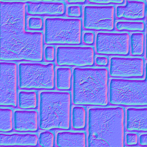
Figure 1: Normal map.
What we end up with is shown in Figure 2. The results are immediately intuitive: areas in the original normal map that were flat are white (glossy), whereas noisy, bumpy sections are darker.
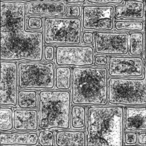
Figure 2: Toksvig map.
With the right kernel size, this Toksvig Map matches up really well against the runtime Toksvig method, which you can see for yourself with the demo at the end. It’s even better under magnification (compare Figure 3a and 3b), as Toksvig AA shows blockiness due to the discontinuous nature of bilinear filtering – cubic interpolation would fix this. (C)LEAN mapping suffers from the same kind of artefacts, but we don’t get this with the baked version because we’ve pre-filtered with a gaussian.
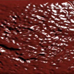
Figure 3a: Toksvig AA under magnification.
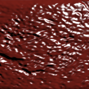
Figure 3b: Toksvig map under magnification.
What we effectively have here is an auto-generated anti-aliasing gloss map, and unlike the (C)LEAN terms, it compresses really well! Also, if this map is generated as part of the art import pipeline, then we’re free to use high precision three-component normals, prior to the compression method of our choosing. So, with this straightforward change, we’ve overcome the two big obstacles of memory consumption and precision.
Using this map is trivial as it’s just like any other gloss map:
1float ft = tex2D(gloss_map, uv).x;
2float p = ft*s;
3float scale = (p + 2)/8;
4float spec = scale*pow(saturate(dot(N, H)), p);
However, the observant reader will notice that the Toksvig Map has been generated with a particular specular power in mind. Fortunately, you can bake with a fixed power that gives reasonable contrast – around 100 seems to work well – and then convert later if you need that flexibility (e.g. for texture reuse or material property changes):
1ft /= lerp(s/fixed_s, 1, ft);Another option is to store the adjusted power, $f_ts$, as the exponent (range [0,1]) of a maximum specular power, as suggested by Naty Hoffman [2]. This log-space glossiness term could be more intuitive for artists to work with and may remove the need for a separate material property for the exponent, plus it’s also a convenient format for direct G-buffer storage [13]. A third option is to store the variance or the length of the normal instead and do the remaining maths at runtime.
The data itself could be packed alongside a specular mask or used to modulate an existing gloss map. I could even imagine the map being used directly as a starting point for artists to paint on top of, but in that case care will be needed to avoid reintroducing aliasing!
Gloss maps are arguably more important than specular masks in the context of physically based shading [2], but artists are typically more comfortable with the latter. Additionally, with the high intensity range that’s possible with energy-conserving specular, anti-aliasing is even more critical. For those reasons, I find the whole idea of an auto-generated texture to be really appealing, even though I haven’t tested all of this out in production yet. I’m a big fan of art tools that do 80-90% of the work automatically, but still provide a way to go in and directly, locally tweak the output. The result is less hair pulling and more time dedicated to polishing. Hopefully this is another example of that.
Gunfight at the O.K. Corral
How does Toksvig Mapping compare to LEAN Mapping? Well, it’s certainly not as good on account of the lack of anisotropy, which can mean over-broadening of the specular highlight in some cases and not enough (leaving dampened aliasing) in others. However, it’s possible to bake CLEAN Mapping instead, which reduces remaining shimmering at the cost of a little more highlight blooming, since it tends to conservatively attenuate.
The reason we can do this is that the main thing separating Toksvig and CLEAN in practice is the measure of variance ($\sigma^2$):
$$ \begin{array}{lcl} \sigma_{toksvig}^2 &=& \frac{1 - |N_a|}{|N_a|}, \\ \sigma_{clean}^2 &=& M_z - (M_x^2 + M_y^2), \\ p &=& \frac{1}{1+s\sigma^2}s. \end{array} $$Everything I already mentioned earlier with respect to Toksvig Maps – baking, evaluating, converting between powers, etc. – applies here too. I’ve even had some success baking LEAN, but I’ll leave talking about that for another time.
Even though LEAN Mapping is closer to the ground truth, baked Toksvig/CLEAN Mapping is still a hell of a lot better than doing nothing, which is precisely what most of us are doing at the moment.
Ride ’em, Cowboy!
Here’s a simple WebGL demo that allows you to toggle between standard Blinn-Phong (default), Toksvig AA and Toksvig Map. You can also edit the shader code on the fly!
Demo update: I’ve had reports of visual issues with the Toksvig Map option and NVIDIA GPUs. If it appears as though you’re missing MIP-maps, then upgrading to the latest drivers (285.62+) should fix the problem.
Besides the shimmering with Blinn-Phong, notice how the teapot remains shiny when you zoom out (mouse wheel) as bumps disappear. In contrast, the material maintains its appearance with Toksvig.
I’ve also created another little example that demonstrates the filtering process.
…Into the Sunset
Phew, that was a rather long post! Perhaps I could have just said: “Store the Toksvig Factor in a texture”, but I enjoyed the journey of getting there and I hope you found it interesting too!
I’ll follow up with more thoughts and an expanded demo at a later date once I’ve had time to investigate further alternatives. In the meantime, I’m interested to hear from anyone who’s explored this area. Besides clearly being a subject that keeps Dan Baker up at night, I spotted that Jason Mitchell had experimented with SpecVar maps [14] for Team Fortress 2 [15] and Naty Hoffman also shared some thoughts on earlier work here [16]. Beyond that though, I haven’t seen much discussion outside of the referenced literature, so I’m all ears!
Acknowledgements
In addition to the great work of all the cited authors, I’d also like to acknowledge sources of inspiration and code for the demo. The live editing environment is (or will be) heavily inspired by Iñigo Quilez’s Shader Toy and Tom Beddard’s Fractal Lab. It makes use of several open source components such as Ace and jQuery, plus various UI widgets. Some WebGL utility code was taken from Mike Acton’s #AltDevBlogADay post, which builds on/refactors this Chromium demo. I’ll save more details on the editor for a future post.
Finally, the normal map is borrowed from RenderMonkey. I trust that this is okay as I couldn’t find a licence anywhere, but please let me know if that isn’t the case. There isn’t a whole lot of freely available data out there and that particular texture, with its rough and smooth areas, makes for a good example.
References
[1] d’Eon, E., Gritz, L., “The Importance of Being Linear”, GPU Gems 3.
[2] Hoffman, N., “Crafting Physically Motivated Shading Models for Game Development”, Physically-Based Shading Models in Film and Game Production, SIGGRAPH Course, 2010.
[3] Baker, D., “Spectacular Specular
- LEAN and CLEAN specular highlights”, GDC 2011.
[4] Persson, E., “Selective supersampling”, 2006.
[5] Filtering Approaches for Real-Time Anti-Aliasing, SIGGRAPH Course, 2011.
[6] Swoboda, M., “Deferred Rendering in Frameranger”, 2009.
[7] Baker, D., “Reflectance Rendering with Point Lights”, Physically-Based Reflectance for Games, SIGGRAPH Course, 2006.
[8] Olano, M., Baker, D., “LEAN Mapping”, I3D 2010.
[9] Donnelly, W., Lauritzen, A., “Variance Shadow Maps”, I3D 2006.
[10] Toksvig, M., “Mipmapping Normal Maps”, 2004.
[11] Kaplanyan, A., “CryENGINE 3: Reaching the Speed of Light”, Advances In Real-Time Rendering, SIGGRAPH Course, 2010.
[12] Pranckevičius, A., “Compact Normal Storage for small G-Buffers”, 2009.
[13] Coffin, C. “SPU-Based Deferred Shading in BATTLEFIELD 3 for Playstation 3”, GDC 2011.
[14] Conran, P., “SpecVar Maps: Baking Bump Maps into Specular Response”, SIGGRAPH Sketch, 2005.
[15] Mitchell, J., Francke, M., Eng, D., “Illustrative rendering in Team Fortress 2”, NPAR 2007.
[16] Hoffman, N., “Lighting Papers”, 2005.
[17] Akenine-Möller, T., Haines, E., Hoffman, N., Real-Time Rendering 3rd Edition, A. K. Peters, Ltd., 2008.