Righting Wrap (Part 2)
Wrapping Paper
I first tinkered with SH wrap shading (as described in part 1) for Splinter Cell: Conviction, since we were using a couple of models [1][2] for some character-specific materials. Unfortunately, due to the way that indirect character lighting was performed, it would have required additional memory that we couldn’t really justify at that point in development. Consequently, this work was left on the cutting room floor and I only got as far as testing out Green’s model [1].
Recently, however, I spotted that Irradiance Rigs [3] covers similar ground. At the very end of the short paper, they briefly present a generalisation of Valve’s Half Lambert model [2] and the SH convolution terms for the first three bands:
$$f(\theta, a) = \left(\frac{\mathrm{max}\left[\mathrm{cos}\,\theta + a,\,0\right]}{1+a}\right)^{1+a}, \\ \quad \mathbf{f} = \left[\frac{2(1+a)}{2 + a},\frac{4(1+a)}{(2+a)(3+a)},\frac{2(1+a)(3-2a+a^2)}{(2+a)(3+a)(4+a)} \right].$$This tidily combines the tunability of [1] with the tighter falloff of [2], albeit at the cost of a few extra instructions in the case of direct lighting. It’s not energy-conserving though, so for kicks I went through the maths – see appendix – and made the necessary adjustments:
$$\hat{f}(\theta, a) = \frac{2+a}{2(1+a)}\left(\frac{\mathrm{max}\left[\mathrm{cos}\,\theta + a,\,0\right]}{1+a}\right)^{1+a}, \\ \quad \mathbf{\hat{f}} = \left[1,\frac{2}{3+a},\frac{3-2a+a^2}{(3+a)(4+a)} \right].$$I would suggest this as a good workout if your calculus skills are a little on the rusty side; think of it as a much-needed trip to the maths gym: sure it’s going to hurt at first, but you’ll feel better afterwards!
The same authors have since written a more in-depth paper, Wrap Shading [4], which Derek Nowrouzezahrai has kindly made available here. I recommend checking it out, since there’s some nice analysis and plenty of background information. One notable insight is that their model is perfectly represented by 3rd-order SH when $a = 1$ (i.e, Half Lambert). This becomes clear when you consider that the model is effectively unclamped in that case, so appropriate scaling of the constant, linear and quadratic bands $(y_{0}^{0}, y_{1}^{0}, y_{2}^{0})$ will match the function:
$$f(\theta, 1) = \left(\frac{\mathrm{cos}\,\theta + 1}{2}\right)^{2} = 0.25 + 0.5\mathrm{cos}\,\theta + 0.25\mathrm{cos^2}\,\theta.$$A similar observation can be made with Green’s model: it’s perfectly represented by 2nd-order SH when $a = 1$.
Shrink Wrap
But wait, at the end of the part 1, didn’t I promise that there would be a discussion of optimisation in this post? You’re quite right. Well, it just so happens that a snippet of reference shader code from this last paper makes for a neat little case study on improving shader performance.
Reference Version
This is pretty much the reference implementation for generating the normalised convolution terms of their generalised model:
 1float3 GeneralWrapSH(float fA)
 2{
 3    // Normalization factor for our model.
 4    float norm = 0.5*(2 + fA)/(1 + fA);
 5    float4 t = float4(2*(fA + 1), fA + 2, fA + 3, fA + 4);
 6    return norm*float3(t.x/t.y, 2*t.x/(t.y*t.z),
 7                       t.x*(fA*fA - t.x + 5)/(t.y*t.z*t.w));
 8}
 9
10float4 main(float fA : TEXCOORD) : COLOR
11{
12    return GeneralWrapSH(fA).xyzz;
13}
The only thing that I’ve changed – beyond adding calling code – is to pass in the wrap parameter fA from the vertex shader. It was previously a user-supplied constant, which doesn’t make for a particularly credible example, since in that case all of the maths could simply be moved to the CPU and performed just the once!
Note that there’s been some attempt to pull out common terms, particularly for the final component, where instead of fA*fA - 2*fA + 3 (see $\mathbf{f}$) we now have fA*fA - t.x + 5.
Without further ado, let’s see how this stacks up in terms of ps_3_0 instructions:
 1//
 2// Generated by Microsoft (R) HLSL Shader Compiler 9.29.952.3111
 3//
 4//   fxc /Tps_3_0 /O3 shader.hlsl
 5//
 6    ps_3_0
 7    def c0, 2, 1, 3, 4
 8    def c1, 0.5, 4, 5, 0
 9    dcl_texcoord v0.x
10    add r0, c0, v0.x
11    add r1.x, r0.y, r0.y
12    mad r1.y, v0.x, v0.x, -r1.x
13    add r1.y, r1.y, c1.z
14    mul r1.y, r1.y, r1.x
15    mul r0.z, r0.z, r0.x
16    mul r0.w, r0.w, r0.z
17    rcp r0.z, r0.z
18    rcp r0.w, r0.w
19    mul r2.zw, r0.w, r1.y
20    mul r1.yz, r0.xxyw, c1.xxyw
21    rcp r0.y, r0.y
22    rcp r0.x, r0.x
23    mul r2.xy, r0.xzzw, r1.xzzw
24    mul r0.x, r0.y, r1.y
25    mul oC0, r2, r0.x
26
27// approximately 16 instruction slots used
Ouch! 16 is fairly substantial, but perhaps not all that surprising going by the HLSL. Since this is device-independent assembly, I decided to check the ALU count on Xbox 360 for comparison. In that case it’s a somewhat more reasonable 10 operations, because 5 scalar ops get dual-issued with vector ops. So, in summary, we have:
DX9: 16, X360: 10(+5) ALU ops
Cancellation
Immediately, a simple but very effective change we can make is to cancel through by the normalisation term, which leaves us with $\mathbf{\hat{f}}$ directly:
1float3 GeneralWrapSH2(float fA)
2{
3    float2 t = float2(fA + 3, fA + 4);
4    return float3(1, 2/t.x, (fA*fA - 2*fA + 3)/(t.x*t.y));
5}
Don’t expect the compiler to do intelligent optimisations like this; constant folding yes, factoring sometimes, sophisticated symbolic manipulation? Good luck!
For instance, even seemingly ‘obvious’ opportunities like (a/b)/(b/a) will go unnoticed by FXC. This isn’t down to the compiler trying to maintain special-case behaviour such as divide by zero either, because it will happily replace a/a with 1 in the absence of any knowledge about the value of a.
Apologies if that was already perfectly clear and all I’ve done is insult your intelligence, but I’ve seen some people blithely leave everything up to the compiler and not scrutinise what it’s generating. Of course, high-level algorithmic optimisations are hugely important as well, but so is this lower-level stuff when a shader is being executed for millions of pixels!
Just look at what this small amount of effort has netted us:
DX9: 10, X360: 5(+3) ALU ops
Factorisation
Next we can factor fA*fA - 2*fA + 3 again – this time as (fA + 1)(fA + 3) - 6*fA – to reduce the numerator of the third term to a single multiply-add:
1float3 GeneralWrapSH3(float fA)
2{
3    float3 t = fA + float3(1, 3, 4);
4    float2 s = t.xy*t.yz;
5    return float3(1, 2/t.y, (s.x - 6*fA)/s.y);
6}
I’ve also taken the opportunity to manually vectorise the addition of fA, plus a subsequent pair of multiplications between resulting terms. In fact, the compiler does this anyway, as it’s relatively good at vectorising code. Still, one shouldn’t assume that it will always get things right!
Whether there’s a gain or not, manual vectorisation – which is often quick to do – makes it easier to sanity check the output assembly. Just scanning through, you might expect add, mul, mov, rcp, mul, mad, rcp, mul and you’d be pretty much spot on.
So, for DX9 we’ve reduced the op count by 2, but what about Xbox 360? Here, we’ve only succeeded in shaving off one paired scalar op. However, this may turn into a real gain once the function is part of a larger shader.
DX9: 8, X360: 5(+2) ALU ops
Rescaling
This next trick involves rescaling so that the second term becomes 1/t.y, or a single rcp:
1float4 c; // {1, 0.5, 1.5, 4}
2
3float3 GeneralWrapSH4(float fA)
4{
5    float3 t = fA*c.xyx + c.xzw;
6    float2 s = t.xy*t.yz;
7    return float3(1, 1/t.y, (s.x - 3*fA)/s.y);
8}
You might wonder why I’m using an external constant here. Well, it turns out that FXC will misoptimise when it knows the values. Bad compiler! Again, there’s one less paired scalar op on Xbox 360:
DX9: 7, X360: 5(+1) ALU ops
Expansion
Rather than factoring terms, we could have expanded $\mathbf{\hat{f}}$ instead:
$$\mathbf{\hat{f}} = \left[1,\frac{2}{3+a},1+\frac{18}{3+a}-\frac{27}{4+a} \right ]=\left[1,0,1 \right ] + \frac{1}{3+a}\left[0,2,18 \right ] - \frac{1}{4+a}\left[0,0,27 \right ].$$
Or in code:
 1float4 c; // {1, 0, 2, 18}
 2
 3float3 GeneralWrapSH5(float fA)
 4{
 5    float2 t = fA + float2(3, 4);
 6    float3 r;
 7    r.xyz  = c.xyx;     // (1, 0,  1)
 8    r.xyz += c.xzw/t.x; // (0, 2, 18)
 9    r.z   -= 27/t.y;
10    return r;
11}
This is a win for ps_3_0 but not for Xbox 360, as it removes the opportunity for pairing. It’s possible that some clever variation could fix this, but it doesn’t matter because we haven’t exhausted our optimisation options…
DX9: 6, X360: 6 ALU ops
Fitting
There are potentially significant gains to be had from numerical fitting, so it’s worth taking the time familiarise yourself with the various techniques, maths packages and libraries out there.
In this instance, I’m performing a cubic fit – i.e. $ax^3 + bx^2 + cx + d$ – for the 2nd and 3rd bands. Polynomials are attractive for performance because they can be efficiently evaluated as a series of mad instructions when written in Horner form: $x(x(ax + b) + c) + d$.
With careful vectorisation, this collapses to the following:
 1float3 GeneralWrapSH6(float fA)
 2{
 3    float4 t0 = float4(-0.018974, -0.052933, 0.076301, 0.208592);
 4    float4 t1 = float4(-0.223994, -0.305659, 0.666667, 0.250000);
 5
 6    float3 r;
 7    r.x  = 1;
 8    r.yz = t0.xy*fA + t0.zw;
 9    r.yz =  r.yz*fA + t1.xy;
10    r.yz =  r.yz*fA + t1.zw;
11    return r;
12}
Xbox 360 does all this in one less operation because placing 1 into r.x can be achieved with a destination register modifier:
DX9: 4, X360: 3 ALU ops
I could present graphs showing how the cubic approximations fare, but take it from me that they are extemely close. In fact, we can arguably drop down to a quadratic fit and save a further mad in the process. This is still acceptable:
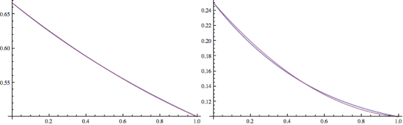
Figure 1: Comparison between original and quadratic fit for 2nd and 3rd bands (left, right).
In both cases – cubic and quadratic – I’ve actually constrained the fitting process so that the curves go through the endpoints. This reduces the worst case error a little and maintains the nice property of exactness when $a = 1$. Of course, something has to give and so the average error is a little higher.
In practice, this quadratic approximation has little effect on the end result. When lighting with a single directional source – a worst-case scenario – the difference is slight and far less significant than the error that comes from using 3rd-order SH in the first place.
Here’s the code for the quadratic version:
 1float3 GeneralWrapSH7(float fA)
 2{
 3    float4 t0 = float4(0.047771, 0.129310, -0.214438, -0.279310);
 4    float4 t1 = float4(0.666667, 0.250000,  0.000000,  0.000000);
 5
 6    float3 r;
 7    r.x  = 1;
 8    r.yz = t0.xy*fA + t0.zw;
 9    r.yz =  r.yz*fA + t1.xy;
10    return r;
11}
DX9: 3, X360: 2 ALU ops
Modifiers
And yet, we’re still not done! The DX9 figure suggests that we might pay the instruction cost of moving 1 into r.x with some GPUs, and although it could go away when the terms are actually used, it would be cute if we could get rid of it just in case.
Notice that the two curves are monotonically decreasing and within the range [0, 1]. If we negate the intermediate result of the first mad, saturate and then negate again, there will be no overall effect. By doing this, we can take r.x along for the ride and force it to 0 through one of the negative constants, then add 1 via the final mad:
 1float3 GeneralWrapSH8(float fA)
 2{
 3    float4 t0 = float4(-0.047771, -0.129310, 0.214438, 0.279310);
 4    float4 t1 = float4( 1.000000,  0.666667, 0.250000, 0.000000);
 5
 6    float3 r;
 7    r = saturate(t0.xxy*fA + t0.xzw);
 8    r = -r*fA + t1;
 9    return r;
10}
Because saturation and negation are typically free register modifiers, we save an operation:
DX9: 2, X360: 2 ALU ops
Going Green
The Wrap Shading paper doesn’t include a normalised version of Green’s model (see part 1), so here’s code for that too:
 1float4 t0; // {0, 1/4, -1/3, -1/2}
 2float4 t1; // {1, 2/3,  1/4,    0}
 3
 4float3 GreenWrapSH(float fW)
 5{
 6    float3 r;
 7    r = t0.xxy*fW + t0.xzw;
 8    r =  r.xyz*fW + t1.xyz;
 9    return r;
10}
DX9: 2, X360: 2 ALU ops
Wrapping Up
Here’s a WebGL sample that encapsulates this mini-series on wrap shading.
In conclusion, shader optimisation is critical for video game rendering, so you shouldn’t defer to the compiler. To quote Michael Abrash: “The best optimizer is between your ears”. Don’t forget it, train it!
References
[1] Green, S., “Real-Time Approximations to Subsurface Scattering”, GPU Gems, 2004.
[2] Mitchell, J., McTaggart, G., Green, C., “Shading in Valve’s Source Engine”, Advanced Real-Time Rendering in 3D Graphics and Games, SIGGRAPH Course, 2006.
[3] Yuan, H., Nowrouzezahrai, D., Sloan, P.-P., “Irradiance Rigs”, SIGGRAPH Talk, 2010.
[4] Sloan, P.-P., Nowrouzezahrai, D., Yuan, H., “Wrap Shading”, Journal of Graphics, GPU, and Game Tools, 15:4, 252-259, 2011.
Appendix
Normalisation factor for generalised Half Lambert:
$$ \begin{array}{lcl} && \frac{1}{\pi}\int_{\Omega}\left(\frac{\mathrm{max}\left[\mathrm{cos}\,\theta+w,\,0\right]}{1+w}\right)^{1+w}\mathrm{d}\omega \\ &=&\frac{1}{\pi}\int_{0}^{2\pi}\int_{0}^{\pi}\left(\frac{\mathrm{max}\left[\mathrm{cos}\,\theta+w,\,0\right]}{1+w}\right)^{1+w}\mathrm{sin}\,\theta\,\mathrm{d}\theta\,\mathrm{d}\phi \\ &=& 2\int_{0}^{\alpha}\left(\frac{\mathrm{cos}\,\theta+w}{1+w}\right)^{1+w}\mathrm{sin}\,\theta\,\mathrm{d}\theta \text{, where }\alpha=\mathrm{cos}^{-1}(-w). \\\\ && \text {Substitute } x=\mathrm{cos}\,\theta,\mathrm{d}x=-\mathrm{sin}\,\theta\,\mathrm{d}\theta: \\ &=& -2\int_{1}^{-w}\left(\frac{x+w}{1+w}\right)^{1+w}\mathrm{d}x \\ &=& \phantom{-}2\int_{-w}^{1}\left(\frac{x+w}{1+w}\right)^{1+w}\mathrm{d}x. \\\\ && \text {Recall that}\int \left(\frac{x+a}{b}\right)^n \mathrm{d}x = \frac{b}{n+1}\left(\frac{x+a}{b}\right)^{n+1} + c: \\ &=& 2\left[\frac{1+w}{2+w}\left(\frac{x+w}{1+w}\right)^{2+w}\right]_{-w}^{1} \\ &=& 2\frac{1+w}{2+w}\left(\left(\frac{1+w}{1+w}\right)^{2+w}-\left(\frac{-w +w}{\phantom{-}1+w}\right)^{2+w}\right) \\ &=& \frac{2(1+w)}{2+w}\left(1-0\right). \\\\ && \therefore \text{ normalise } f(\theta, w) \text{ with } \frac{2+w}{2(1+w)}. \end{array} $$